Minimizing Uncertainty
In many engineering disciplines designs are based on the performance of “man-made” products, while geotechnical engineers design from measured properties of soil or rock materials placed at the site by “mother-nature.” In this context, the geotechnical engineer should choose the most accurate analytical model for his/her design to best predict the outcome or performance of the structure. The geotechnical engineer must use tests that accurately measure the soil or rock properties to input into his/her design model. Failmezger and Bullock (2008) present a series of guidelines, e.g., “Which in-situ test should I use—a designer’s guide.”, to streamline this process. The engineer should avoid using a perhaps “cheaper” test and correlate soil/rock properties with more accurate/specific tests for design. The low-cost testing approach only creates additional, undesired layers of uncertainty. The engineer should specifically use the more accurate testing for design, and use the “cheaper” testing for simpler objectives, such as identify soil strata, profiling of critical layers, or pinpointing locations at the site that need accurate testing.
From a statistical viewpoint, soil/rock properties tend to follow the central limit theory of probability, where values cluster near their average forming a “bell-shaped” distribution. Duncan (2001) suggests that the minimum or maximum value occurs three (3) standard deviations from the average value. As an estimate of standard deviation, Duncan suggests for the engineer to determine what the largest and smallest value of those properties can be and divide their difference by 6. Wickremesinghe (1989) and Uzielli (2008) show methods to statistically analyze geotechnical data.
Because of uncertainty, the soil or rock property is not a fixed value, but falls within a “bell-shaped” probability distribution of values. Factor of safety approaches for geotechnical design incorrectly assume that the soil/rock properties and the minimum design factor of safety values have constant values and do not consider the natural or spatial variability of those properties throughout the site, how well the engineer measures or knows what those values are, or the owner’s financial risk. Mathematicians have made this concept much more difficult than it is, regrettably causing engineers to shy away from probability analyses for design. Failmezger (2018) discusses further in his technical paper, Quantifying Geotechnical Probability of Failure—a Simpler Approach. Engineers only need to know that the area under a probability distribution curve must always equal 1.0. Why? There is 100% certainty that the value lies within this range, making its area equal to 100% or 1.0. The engineer can determine the likelihood or probability that its value will exceed “x” by simply summing the area under the curve to the right of “x” or determine the probability that its value will be less than “x” by simply summing the area under the curve to the left of “x”.
Because of readily available tables of solutions, many researchers have suggested using either a “normal” or “log-normal” probability distribution. Unfortunately, the “normal” distribution has end limits that range from negative infinity (-∞) to positive infinity (+∞) and the “log-normal” distribution has end limits from just more than zero to positive infinity (+∞). Both distributions have non-representative end limits for engineering design. Fortunately, the “beta” probability distribution has end limits that the engineer chooses and best represents geotechnical engineering design (at least in our opinion) as documented by Failmezger, Bullock and Handy (2004) – Site, variability and beta. To compute the beta probability distribution function, the engineer must input the minimum end limit value, the maximum limit value, the average value and the standard deviation. The beta probability distribution function uses the following equation:
Note Excel factorial function only computes whole numbers, while older HP calculators computed the factorial correctly for non‐integers.
The engineer can easily check the correctness of the equation by summing the area underneath it using a numerical method such as the trapezoidal method. Excel spreadsheets for slope stability (Figure 1), pile capacity (Figure 2), settlement (Figure 3) and angular distortion make probability computations relatively routine. These spreadsheets show the equation for the beta probability function and include sum of the area check for correctness.
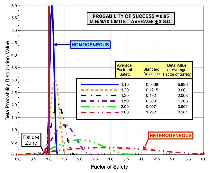
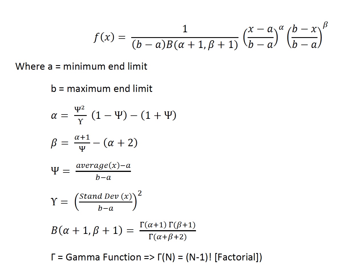
Figure 1: Beta Probability Distribution Functions for Probability of Success = 95%
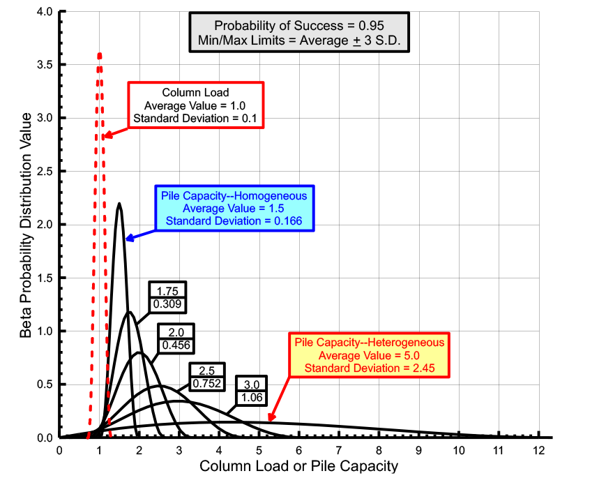
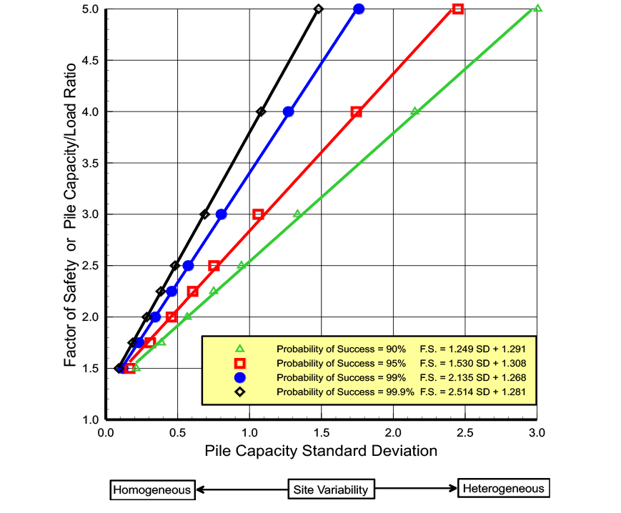
Figure 2: Beta Distribution Curves with
Load Curve with Standard Deviation of 0.1
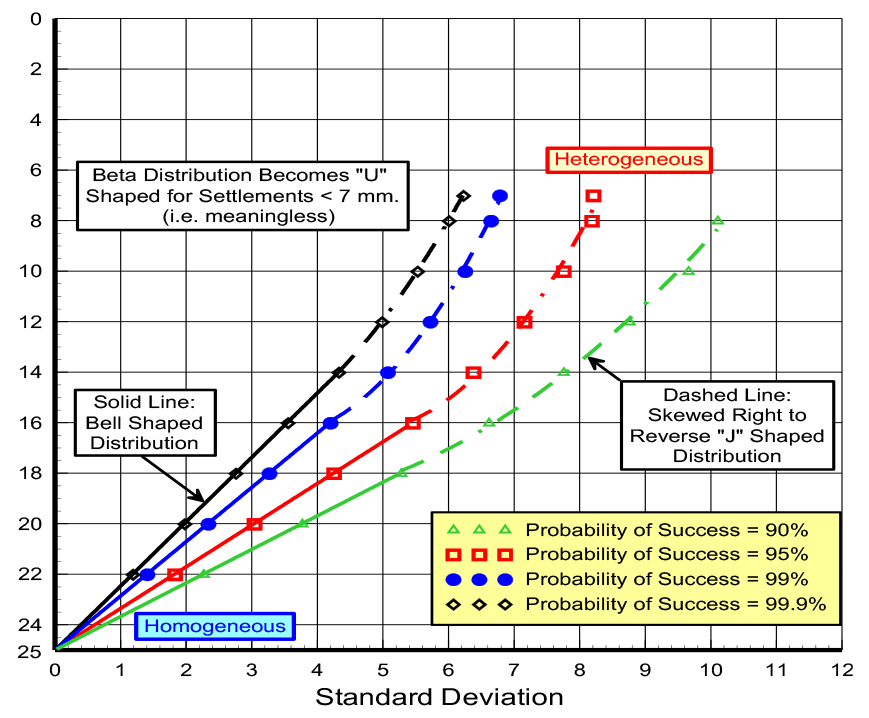
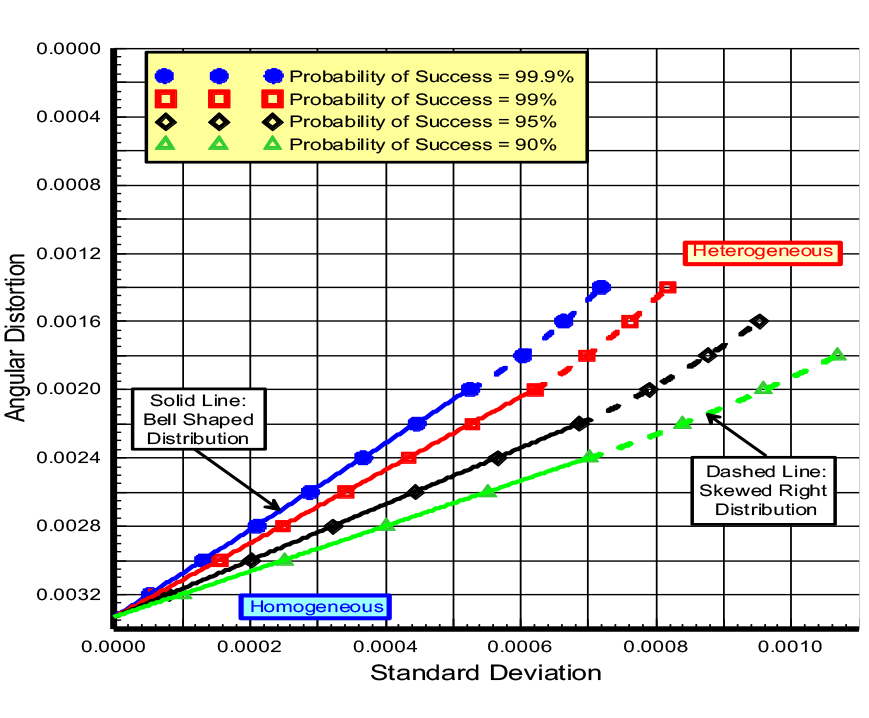
Failmezger has developed design charts graphing and summarizing the probability distribution solutions for the above geotechnical engineering designs (Figure 4a-d).
Figure 3: Beta Probability Distribution Curves for Settlement
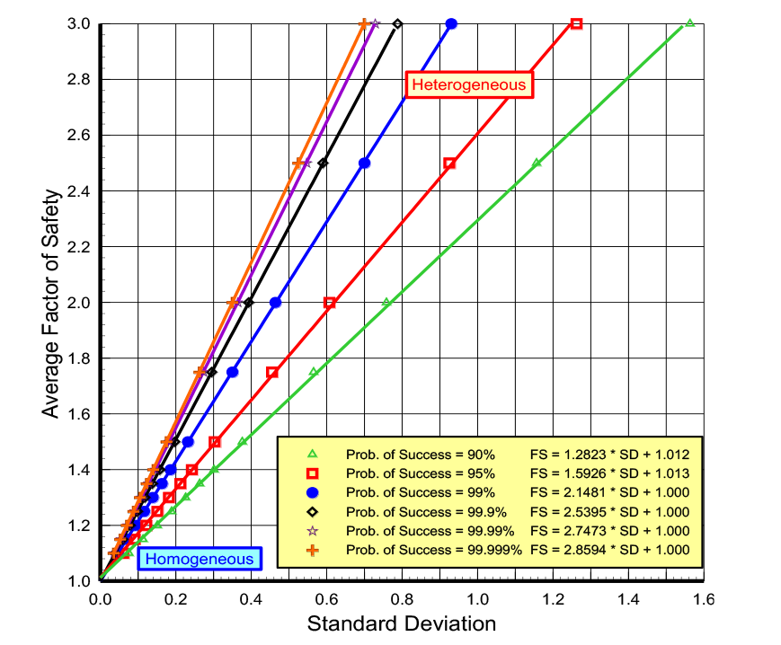
The property’s standard deviation represents uncertainty—low uncertainty has low standard deviations while high uncertainty has high standard deviations. With accurate measurements, the probability distribution function for the soil or rock property becomes narrow and steep, because its values fall within the narrow band centered around its average value with low standard deviations and end limits close to the average value. In this case the probability distribution curve is steep and narrow. On the other hand, where the soil or rock property has high uncertainty, the resulting probability distribution curve becomes wide and short to cover the wide range of potential values (Figure 5).
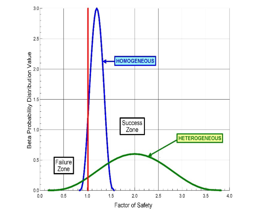
Figure 5: Probability of success=0.95 for both homogeneous and heterogeneous uncertainties
The engineer can compute the standard deviation from three sources of uncertainty:
- the site or spatial variability of the soil/rock properties,
- the accuracy of the prediction method, which can be computed from case study databases,
- and other intangible sources based on engineering judgment.
If the engineer views these three sources of standard deviation as independent of each other, then the overall standard deviation equals:
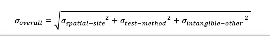
The overall standard deviation will decrease if these sources of uncertainty have some dependence with each other.
Often, geotechnical engineers recommend a single allowable bearing capacity for all shallow spread footings or a single pile tip elevation for all deep foundations to support the proposed structure. Even if the soil has exactly the same deformation modulus for the entire site, different column loads will mathematically cause differential settlement. Smaller column loads have smaller stress bulbs, while larger column loads have larger stress bulbs. For a constant deformation modulus of 100 bars, Failmezger shows in Figure 6 that larger stress bulbs result in larger settlements for the larger applied column loads.
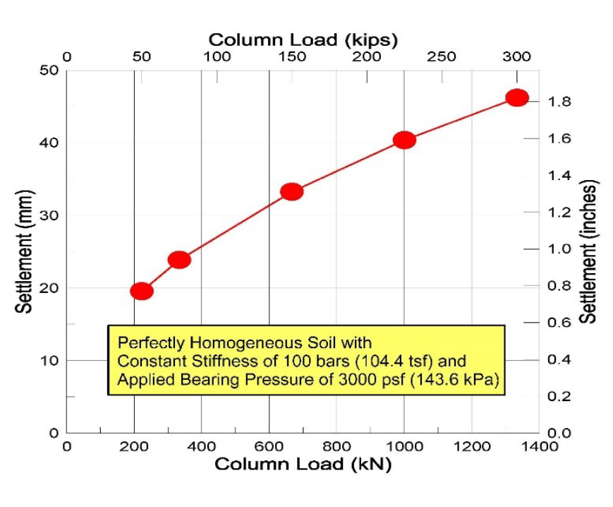
Figure 6: For same stiffness and applied bearing pressure—more settlement for larger loads
Ideally, for the best performance of the structure, the geotechnical engineer would design so that each shallow spread footing settled the same amount or each deep foundation pile or pier supports the same applied load. Failmezger and Bullock (2004) present guidance in their technical paper, Individual Foundation Design for Column Loads. Failmezger and Niber (2006) present a case study using accurate dilatometer test data to predict settlement and probability analyses to design a shallow foundation system for a parking garage for Washington D.C. metro system. The owner should be involved in making risk decisions for the foundation design solution, as Failmezger and Bullock discuss in Owner Involvement–Choosing Risk Factors for Shallow Foundations.
Engineering design should consider two types of failure: 1) failure of the structure to perform satisfactorily and 2) financial failure—the owner’s additional and unnecessary costs from overly-conservative designs as a result of high uncertainty in the soil or rock properties (Figure 7). The engineer should balance these two sources of failure by making accurate measurements of the soil or rock properties, resulting in an accurate, safe and cost-efficient design. Failmezger (2021) explains further the additional cost that the owner will have if the geotechnical engineer does not design based on thorough knowledge of the soil or rock properties at the site in his technical paper, “Financial Failure—The High Cost of Not Knowing”. Brumund (2011) discusses business risks for geotechnical engineering firms.
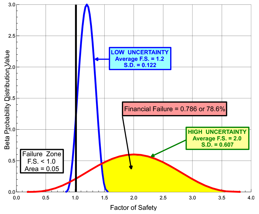
Figure 7: Financial Failure Calculating Risk