Geotechnical Design Method Quantifying Risk —Probability of Success Analyses

In many engineering disciplines, designs depend on a relatively narrow range of properties of “man-made” products, while geotechnical engineers design measuring properties of soil or rock materials placed at the site by “mother-nature” that often vary significantly. The geotechnical design engineer has traditionally used a factor of safety approach that incorrectly assumes that the soil/rock properties and the minimum design factor of safety values have constant values. Because of uncertainty, the soil or rock properties do not have fixed values, but rather fall within a “bell-shaped” probability distribution of values. Design uncertainties dictate the shape of this curve—low values have steep and and narrow curves, while large values have flat and wide curves and costs more to construct. These uncertainties include 1) the natural or spatial variability of those properties throughout the site, 2) how well the engineer measures or knows what those values are, and 3) how well the design method predicts the outcome.

The geotechnical engineer should choose the most accurate analytical model for his/her design to best predict the outcome or performance of the structure. Less accurate tests with high uncertainty may falsely cause the design engineer to think that the site has more variability than it does. Therefore, the geotechnical engineer must use tests that accurately measure the soil or rock properties to input into his/her numeric design model. Failmezger and Bullock (2008) present guidelines, e.g., “Which in-situ test should I use—a designer’s guide.”

Soil property correlations based on less accurate tests have an additional or fourth source and undesired layer of uncertainty. To minimize this uncertainty, the engineer should compare values from the less accurate tests with values from the accurate tests and develop “site-specific” correlations. How good are those correlations? If the correlation poorly matches the accurate data, then its standard deviation will have large value, making the design standard deviation unnecessarily high. In this case, the engineer may decide to discard the less accurate tests all together from the design analyses and simply base the design on the accurate tests.

For example, the engineer may correlate the SPT N60 value, which ranges from 1 to 50 blows per foot, or CPT qt, which ranges from 1 to 500 tsf, with the deformation modulus from dilatometer or pressuremeter tests for design of settlement for shallow foundations. (The SPT torque measurement has a resolution approximately 10 times N60, and thus can significantly improve SPT correlations.) Unfortunately, both the SPT and CPT strain the soil to failure, while the proposed structure strains the soil to an intermediate level, as do the dilatometer and pressuremeter. Strain incompatibility may lead to high correlation error and uncertainty.

Mathematicians have made probability analysis seem much more difficult than it is, regrettably causing engineers to shy away from using it for design. Engineers only need to know that the area under any probability distribution curve must always equal 1.0. Why? There is 100% certainty that the value lies within this range, making its area equal to 100% or 1.0. If one flips a coin, it will land as either a head or tail. While one does not know whether it land as a head or tail, one of those two outcomes will occur. Similarly, if the weather prediction calls for 30% of rain, then it also calls for a 70% chance that it will not rain. But there is a 100% chance that it will either rain or not rain. With engineering, a desirable outcome will occur at a certain percentage (probability of success) and one minus that percentage that an undesirable outcome will occur (probability of failure). Failmezger (2018) discusses this topic further in his technical paper, Quantifying Geotechnical Probability of Failure—a Simpler Approach.

Historically, geotechnical design has an average probability of success of about 95% (Harr, 1977 and Duncan, 2000). With a probability analysis, the geotechnical engineer quantifies the owner’s desired probability of a successful outcome. As the probability of success increases, the owner’s cost increases. The owner balances the initial construction cost with the potential repair cost. For example, an owner building a warehouse may choose a probability of success of 90%, while an owner building a hospital may choose a probability of success of 99%.

From a statistical viewpoint, soil/rock properties tend to follow the central limit theory of probability, where values cluster near their average forming a “bell-shaped” distribution. Duncan (2000) suggests that the minimum or maximum values occur three (3) standard deviations from the average value. As an estimate of standard deviation, Duncan further suggests for the engineer to determine the largest and smallest possible values of those properties and divide their difference by 6. Wickremesinghe (1989) and Uzielli (2008) show methods to statistically analyze geotechnical data.

Many researchers have suggested using either a “normal” or “log-normal” probability distribution because tables established more than 50 years ago provide numerical solutions. Unfortunately, the “normal” distribution has end limits of negative infinity (-∞) to positive infinity (+∞) and the “log-normal” distribution has end limits from just more than zero to positive infinity (+∞). The computed area of the failure zone (between 0.01 and 0.1 for a probability of success equal to 99% and 90%, respectively) lies within one of the tails of the probability distribution curve and thus the end point becomes critical for this computation. Both normal and log-normal distributions have non-representative end limits for engineering design.

Fortunately, the “beta” probability distribution has end limits that the engineer chooses and therefore best represents geotechnical engineering design as documented by Failmezger, Bullock and Handy (2004) – Site, variability and beta. Using Excel with its built-in functions, the engineer can compute the beta probability distribution function. The engineer can and should check the correctness of the equation by summing the area underneath the probability distribution curve using a numerical method such as the trapezoidal method. This area must equal 1.000. To solve the equation for the beta probability function, the engineer must evaluate and input the minimum end limit value, the maximum end limit value, the average value, and the standard deviation.

The beta probability distribution function has the following equation:

Formula

Using the beta probability function, the engineer can solve:

  • factor of safety analyses,
  • driving forces/resisting forces analyses (pile capacity, tiebacks, slope stability, retaining walls), and
  • settlement or angular distortion analyses.

Failmezger solved these problems using Excel spreadsheets and summed the area under the probability curves proving correctness (area = 1.00). Figures 1-3 show those beta probability distribution functions. Summary graphs of these solutions let the design engineer more easily perform a probability analyses without necessarily solving the above equations.

The engineer selects the average values and standard deviations for the geotechnical parameters for the design life of the project. The input parameters in the probability analyses do not include time, and the probability of success represents time equal to the design life that the engineer/owner chooses.

Beta Probability Distribution Functions for Probability of Success = 95%
Beta Distribution Curves with Load Curve with Standard Deviation of 0.1
Beta Probability Distribution Curves for Angular Distortion = 1/150
Beta Probability Distribution Curves for Angular Distortion = 1/300
Beta Probability Distribution Curves for Angular Distortion = 1/500
Beta Probability Distribution Curves for Angular Distortion = 1/750

Factor of Safety Analyses

Christian (1997) developed his point estimate method to analyze the factor of safety probability analyses. For each geotechnical design parameter, the engineer selects either its average value plus one standard deviation or its average value minus one standard deviation. The engineer then performs 2n analyses, where n = the number of parameters. So, if the engineer has four parameters, he/she would run 24 or 16 analyses. From this data set for factor of safety analyses, the engineer can determine the average and standard deviation. With this analysis, the engineer can readily find which parameters have the most influence on the design.

Design Chart for Factor of Safety with end limits = average + 3 standard deviations
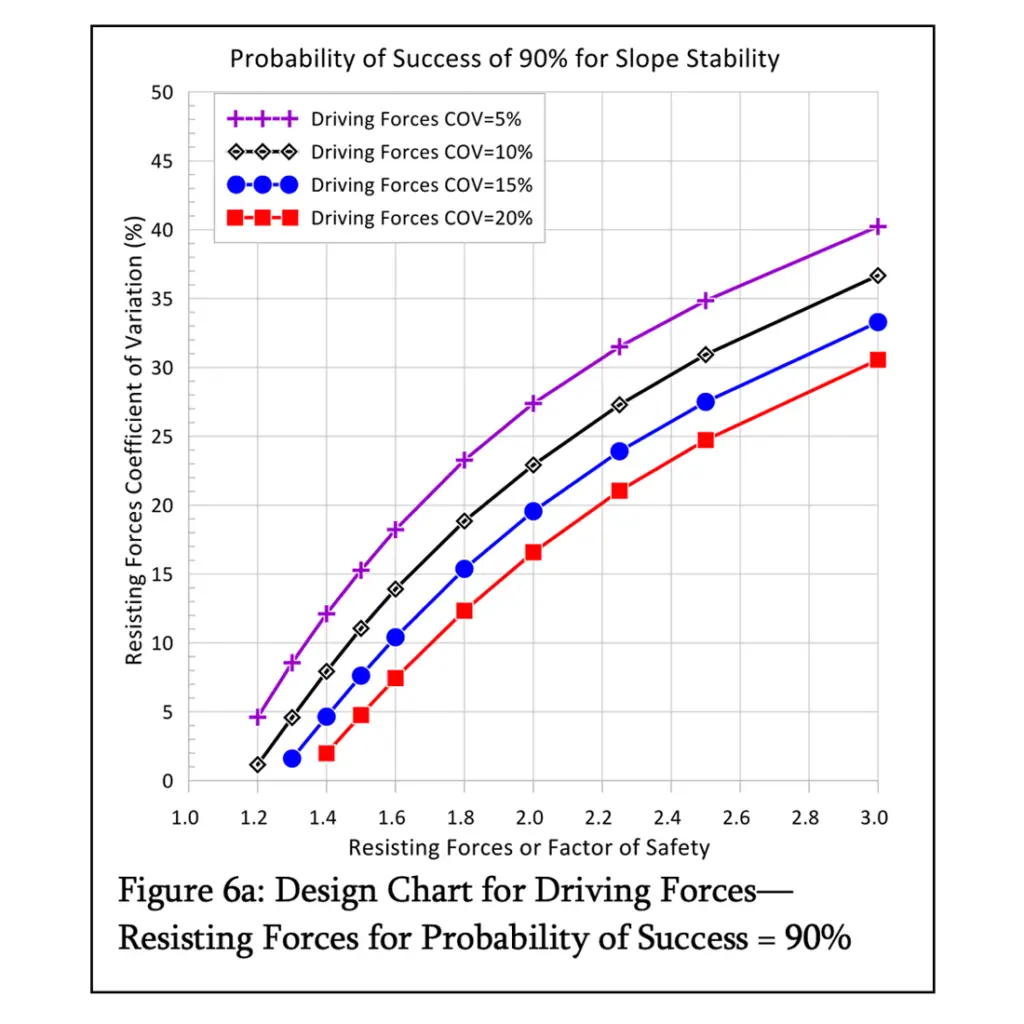
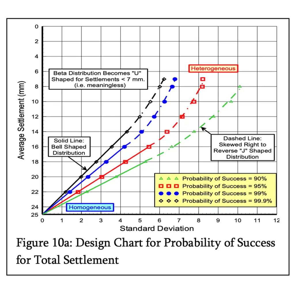
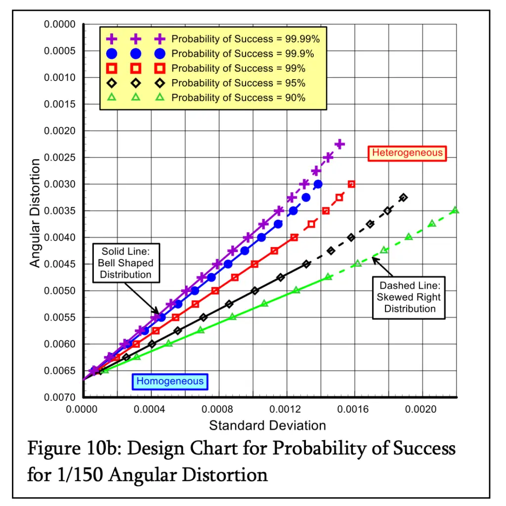
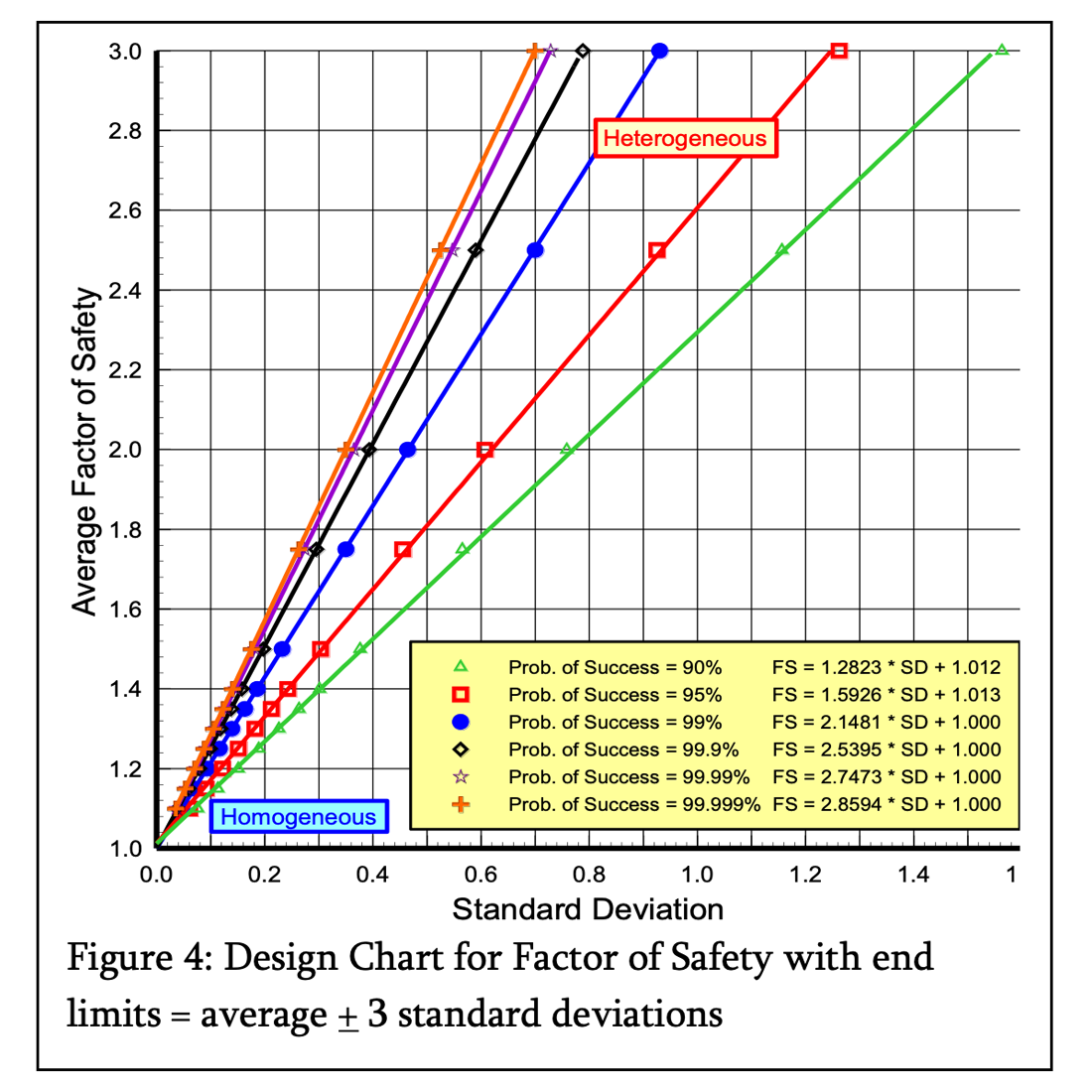
By assuming an average value of factor of safety and end limits three standard deviations away from the average, Failmezger, Bullock and Handy computed the standard deviation that gave probabilities of success equal to 90, 95, 99, 99.9, 99.99 and 99.999%. Interestingly, the average factor of safety versus standard deviation has a linear relationship for different probabilities of success. Although Dr. Dick Handy told Roger Failmezger that some terms would cancel out when Failmezger tried to mathematically solve the problem at Dick’s breakfast table, he unfortunately ended up with a sixth order polynomial equation with all the terms. While the engineer can solve for the probabilities of success of 99.9, 99.99, and 99.999%, he/she is likely “slicing the bologna simply too thin” as the geotechnical parameters for the analyses are not known that accurately. After determining the average factor of safety and the standard deviation, the engineer can use the design chart shown as Figure 4 to determine its probability of success. The engineer adjusts the design to get the desired probability of success that the owner selects. 

Driving Forces—Resisting Forces Analyses

The engineer can design for slope stability, lateral and vertical capacity of deep foundations, tiebacks, and retaining walls using the driving forces/resisting forces analyses. By assigning a value of 1.0 as the average value for the driving forces, the analyses simplify and become unitless. The coefficient of variation equals the standard deviation divided by the average value. By assuming a coefficient of variation of either 5, 10, 15 or 20% for the driving forces and an average value of either 1.2, 1.3, 1.4, 1.5, 1.6, 1.8, 2.0, 2.5 or 3.0 for the resisting forces, Failmezger determined the coefficient of variation for the resisting forces to get a probability of success equal to either 90, 95, or 99%.

By separating the driving and resisting forces, the engineer can often better estimate their coefficients of variation than the overall coefficient of variation for a factor of safety analyses that combines these forces. For a slope stability problem, the engineer can perform his/her routine factor of safety analysis with computer software because the computed minimum factor of safety across the critical failure surface equals the average resisting force when assuming the average driving force equals 1.0. Figures (5a-d) provide solutions for the probability of success, after the engineer chooses the appropriate coefficient of variation for driving forces chart and evaluates the average value and coefficient of variation for the resisting forces. For example, if the COV for the driving forces = 5% and COV for the

Design Chart for Driving Forces with a Coefficient of Variation = 15%
Design Chart for Driving Forces with a Coefficient of Variation = 10%
Design Chart for Driving Forces with a Coefficient of Variation = 20%

resisting forces = 15%, then the average resisting force or factor of safety would need to equal 1.4 for a probability of success = 90%, 1.5 for a probability of success = 95%, or 1.7 for a probability of success = 99%.

After communicating with the owner and other design team members, the geotechnical design engineer may know the desired probability of success for the project. Figures 6a-c show the probability of success of 90, 95, and 99% for the driving forces—resisting forces analyses.

Design Chart for Driving Forces—Resisting Forces for Probability of Success = 90%
Design Chart for Driving Forces—Resisting Forces for Probability of Success = 95%
Design Chart for Driving Forces—Resisting Forces for Probability of Success = 99%

Settlement—Angular Distortion Analyses

For this analysis, the geotechnical design engineer determines the probability that the predicted settlement will be less than the chosen threshold total settlement or angular distortion for the structure. The engineer should perform deformation tests for his/her settlement prediction method, such as flat dilatometer or pressuremeter tests (Figure 7). Settlement predictions based on penetration tests (SPT and CPT) that strain the soil to failure can have inaccurate and high standard deviation or coefficient of variation for useful probability analyses (Figure 8).

Dilatometer tests to predict settlement (COV of method = 0.18)
Predicted Settlement (mm)

Figure 9 shows the Beta probability distribution functions for settlement and angular distortion. Notably, when the standard deviation has a low value, the curves have a bell-shape and closer to the threshold value, while when the standard deviation has a high value and the minimum end limit becomes zero, the curves become skewed right then “reverse J-shaped” and farther from the threshold value.

Total Settlement
Angular Distortion = 1/300

Foundation design minimizes the settlement difference between any two columns for the structure relative to the distance between them, or the angular distortion, to avoid unacceptable damage to the structure. Table 1 shows limits of angular distortion for different types of structures and their uses. The geotechnical engineer, the owner and structural engineer, working closely together, should choose the appropriate risk levels for the desired angular distortion of the structure.

Table 1 Allowable Angular Distortion

Situation Allowable Angular Distortion
Machinery sensitive to settlement
1/750
No cracking in buildings; tilt of bridge abutments; tall slender structures such as stacks, silos, and water tanks on a rigid mat; steel or reinforced concrete frame with brick block, plaster or stucco finish and length to height ratio greater than 5
1/750
Cracking in panel walls; problems with overhead cranes
1/750
Structural damage in buildings; flexible brick walls with length to height ratio greater than 4
1/750

Figures 10a-e present design charts for total settlement and angular distortion of 1/150, 1/300, 1/500 and 1/750 plotting their average value versus standard deviation to determine the design probability of success.

Design Chart for Probability of Success for Total Settlement
Design Chart for Probability of Success for 1/300 Angular Distortion
Design Chart for Probability of Success for 1/500 Angular Distortion
Design Chart for Probability of Success for 1/750 Angular Distortion

Standard Deviation
The standard deviation measures the design uncertainty. When the engineer minimizes the standard deviation in his/her design, the solution results in a steep and narrow shaped probability distribution (blue) curve. However, high standard deviation results in a short and wide shaped probability distribution (green) curve, as illustrated on Figure 11.
When the engineer evaluates the standard deviation, he/she should consider three sources of uncertainty:

  1. the site or spatial variability of the soil/rock properties and foundation loads,
  2. the accuracy of the prediction method, which can be computed from case study databases,
  3. and engineering judgment to evaluate other intangible sources.
Blue curve => low uncertainty Green curve => high uncertainty

If the engineer views these three sources of standard deviation as independent of each other, then the overall standard deviation equals:

Formula: Standard deviation

If the engineer correlates less accurate test data with accurate data, then the standard deviation from “site-specific” correlation contributes to the overall standard deviation as follows:

Formula: Standard deviation

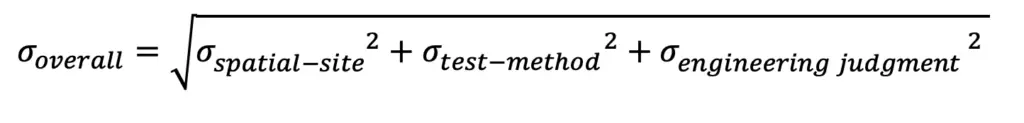
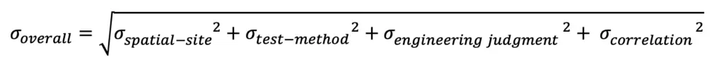
The overall standard deviation will decrease if these sources of uncertainty have dependency with each other.

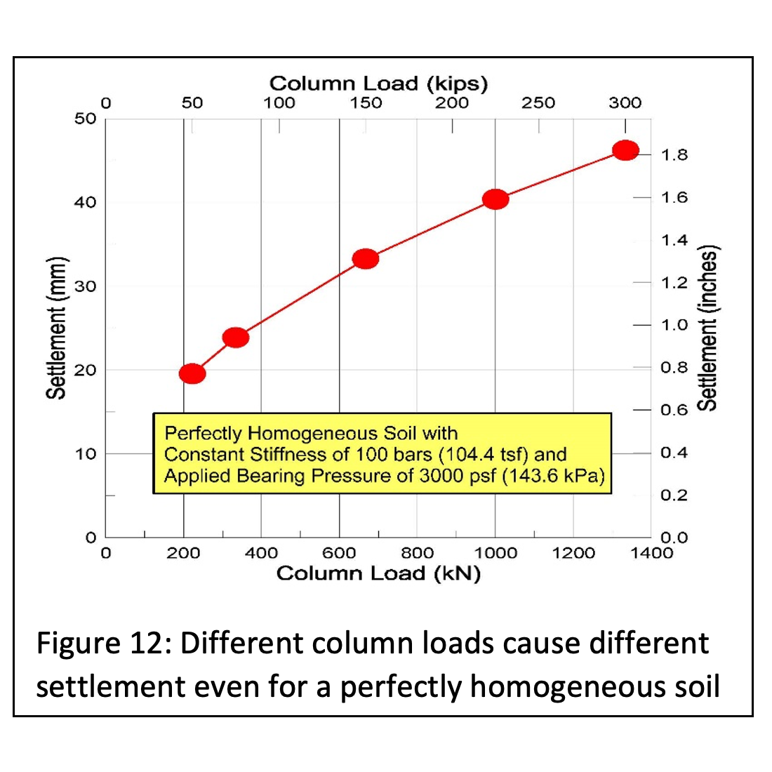
Site/spatial variability: After a thorough subsurface investigation, the geotechnical engineer should assess the variability of soil/rock properties. Are they homogeneous and therefore represented with a low standard deviation?Different column loads cause different settlement even for a perfectly homogeneous soil Or does the site have differing properties? Are the column loads similar for the entire structure or do they differ? Unfortunately too often, geotechnical engineers overly simply design and recommend a single allowable bearing capacity for all shallow spread footings to support the proposed structure. Even if the soil has exactly the same deformation modulus for the entire site (perfectly homogeneous), different column loads will mathematically cause differential settlement. Smaller column loads have smaller stress bulbs, while larger column loads have larger stress bulbs. For a constant deformation modulus of 100 bars, Failmezger shows in Figure 12 that larger stress bulbs result in larger settlements for the larger applied column loads.

For the best performance of the structure, the geotechnical engineer designs each shallow spread footing to settle the same amount or each deep foundation pile or pier to support the same applied load. To get the same settlement for spread footing design, the geotechnical engineer should use higher bearing pressures for smaller loads and lower bearing pressures for higher loads. To achieve uniform settlement for the site using ground improvement to increase the deformation modulus, the soil should be improved more at the higher column loads and less at the lower column loads. For deep foundations, the geotechnical engineer should compute the tip depth and number of piles or piers to provide the predicted capacity equal to the column load times the factor of safety. For example, at a column instead of computing 8.2 piles and installing 9 piles, install 8 piles a foot or two deeper.

Each test hole becomes a settlement or pile capacity prediction. By plotting these points as a contour map of settlement for spread footings or tip depth for deep foundations, the engineer can visualize how the structure will perform. Holes or hills on the contour map represent areas where there are insufficient data and more testing should be performed at the center of those uncertain zones. Failmezger and Bullock (2004) present guidance in their technical paper, Individual Foundation Design for Column Loads. For columns that do not have a test hole at their location, the engineer can use a weighted average to predict the settlement of the spread footing at that column. From the settlement predictions from three holes (A, B, and C) closest to that column, the geotechnical engineer computes the weighted average using the following formula:

SettCol Formula

Where SettCol = the weighted average prediction for settlement at center of column
DistA = the distance from hole A to the center of column

SettA Formula

The holes closest to the column have more “weight” or influence on the settlement prediction of the column. Similarly, the geotechnical engineer can predict the tip depth for the deep foundation at each column using the above weighted average formula.

With this approach to design for the support of each column individually, the geotechnical engineer minimizes the uncertainty from the spatial variability of the soil/rock and loads. Each prediction at a column becomes a data point in the set used to compute the average and standard deviation for the design. To minimize the site’s spatial variability, the geotechnical engineer adjusts the design as the load and geotechnical properties change across the site.

Failmezger and Niber (2006) present a case study using accurate dilatometer test data to predict settlement and probability analyses to design a shallow foundation system for a parking garage for Washington D.C. Metro Transportation Authority (WMATA). WMATA, a conservative owner, accepted a shallow spread footing design that had a probability of success of 93% that footings would settle less than 1.0 inch. WMATA saved a significant amount of money with this design and today the parking garage performs as desired. The owner should always be involved in making risk decisions for the foundation design solution, as Failmezger and Bullock discuss in Owner Involvement–Choosing Risk Factors for Shallow Foundations.

The geotechnical engineer can use histograms to visualize the variability and average value for soil/rock properties for each geologic formation. Stark (2024) shows a histogram for liquid limit of a clay at a site on Figure 13. If the engineer observes two distinct centers of data, then he/she should separate data into two different soil/rock layers in the analyses. The standard deviation can be computed as dividing the difference between the maximum and minimum values by 6 as suggested by Duncan (2000).

Histogram of liquid limit

Design Method Variability: How well does the design method predict the outcome? Well documented case studies can give the engineer the coefficient of variability for the design method/outcome. When Failmezger asked Dr. John Schmertmann about predictions, he emailed “I remember that MIT professor Bill Lambe was very interested in predictions and tried to put them in categories like A —meant the predictor was completely unaware of the correct answer, and B – knew the answer, with various nuances in between”. Briaud (2012) describes predictions as accurate meaning that the average prediction matches the average measurement and precise meaning that there is little scatter or low standard deviation in the prediction.

From Schmertmann (1986) and Hayes (1986) data sets shown on Figure 7, settlement predictions for spread footings from dilatometer are both accurate and precise, having a low coefficient of variation of 0.18. For slope stability analyses, the Morganstern-Price 3-dimensional method has a closed form solution, minimizing its coefficient of variation. From pile load tests, Robertson, et. al. (1988) shows that the LCPC method using CPT data has a coefficient of variation equal to 10% for driven steel pipe piles.
From performance monitoring during load tests at the site and regionally in a specific geologic formation, the geotechnical engineer can compute the coefficient of variation for the method. To learn, the geotechnical engineer should always carry out pile load tests to failure. From the instrumentation, such as strain-gauge sister bars, the engineer computes the ultimate resistance unit stresses for each stratum along the test pile.

The geotechnical engineer can perform conical test load (Schmertmann 1996) or embankment load tests to improve/evaluate the settlement method prediction variability for the site. The conical test load method places a cone shaped mound of gravel over the supporting soil, imposing the stress that the spread footing will apply. Using settlement plates and stress cells, the engineer models how a spread footing will perform.
He/she then adjusts the correlation coefficients for each stratum in the prediction method to match the load test. Stark (2024) describes these adjustments as “anchoring the correlation”.

Engineering judgment variability:
Time and budget constraints may limit the design engineer from obtaining enough test data to accurately and precisely perform his/her design. The design engineer may not have performance tests to improve the design. The engineer may not observe the construction of the project to assure that it is built as designed. Supporting footings on previously placed but undocumented fill represent high uncertainty. Even with a significant number of test holes, soft, loose, debris, and organic material may not be discovered with the field explorations. The seasoned engineer assesses these potential uncertainty sources and evaluates their impact for an unsatisfactory outcome.

Choosing the Probability of Success
The engineer must perform design services to meet the standard of care, i.e. the level of service provided by an average engineer in the geographical area at the time of service. The engineer carries professional liability insurance that covers the risk only when his services do not satisfy the standard of care. The geotechnical engineer includes a risk disclaimer flyer in his/her report trying to deflect responsibility if a performance failure occurs. Juries for court cases tend to find the engineer at least partially responsible because “they said it would work” in their design report and it did not. To protect themselves, today’s engineers tend to design overly conservatively and costly to the owner.

Successful owners make money. They maximize their profits by seeking a foundation design that safely supports their structure and costs the least to build. They choose the probability of success that balances the risk of performance failure with the risk of financial failure.

The engineer and owner must discuss risk. With this approach, the owner chooses the risk for the project and the engineer quantifies and designs for the chosen desired risk or probability of success.

Financial Failure from Poor Quality Data
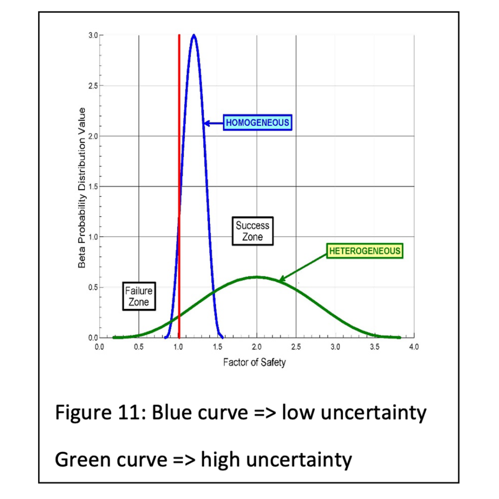
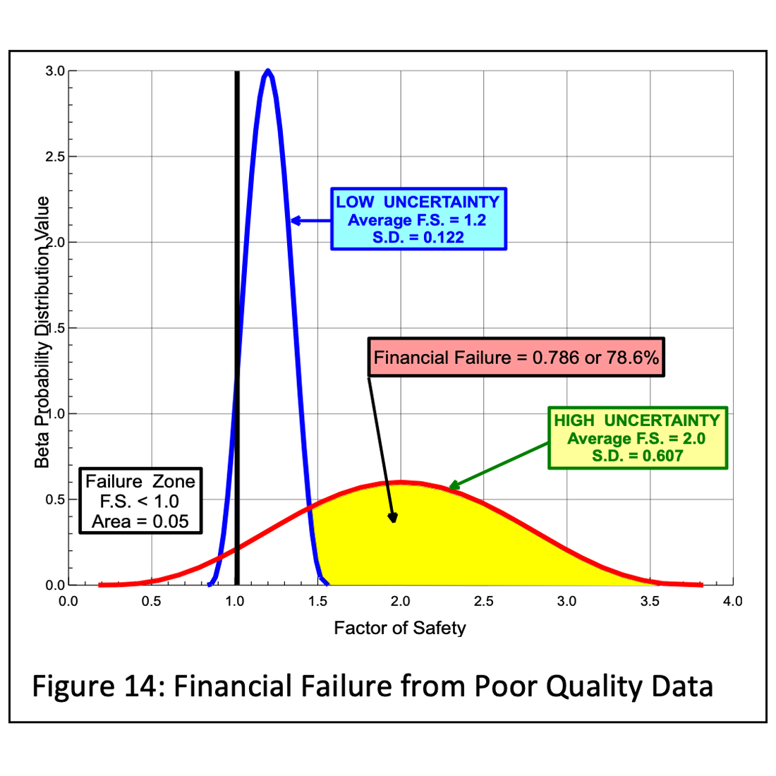
To minimize his/her risks, the owner should select the engineer based on his/her qualifications rather than fees. To minimize uncertainty and the design risks, the engineer accurately and thoroughly measures the soil/rock properties. The resulting design curve becomes steep and narrow as depicted as the blue curve on Figure 14. If the engineer does not make enough accurate measurements of the soil/rock properties, he/she cannot determine whether the resulting high uncertainty is attributed to variability of the soil/rock properties or his/her lack of knowledge. In this case, the resulting design curve becomes shallow and flat as depicted as the red curve. Both curves represent a probability of success of 95%. If the engineer’s design results in the red curve because of a lack of knowledge instead of the blue curve, then where the red curve exceeds the blue curve, that area computes as the probability of financial failure. The wise owner would spend money on a more thorough soil property investigation and engineering design resulting in the low uncertainty (blue) curve design.

High Risk—Non-Redundant Foundation Systems: When foundation systems have a single drilled shaft supporting a column or the owner wishes to minimize all risks, Schmertmann and Schmertmann (father/son), 2012 developed the Testing and Remediation Observational Method (TROM). With TROM, the engineer tests every foundation to ensure that it has the capacity to provide the support needed to carry the load. When a tested foundation does not have enough capacity, then it is remediated until it has that capacity. TROM successfully proved the adequacy for foundation system for the Los Angeles Football Stadium in 1995 and routinely verifies capacity for tieback support systems.

The owner must decide what probability of success is best for his/her project. Historically, the average probability of success is about 95% (Harr, 1977 and Duncan, 2000). What is the cost to repair a performance failure? If it is high, then the design should use a higher probability of success. If it is low, then the design should use a lower probability of success. For example, a crack in the foundation or slab in a warehouse, which may not be repaired, has less importance than a crack in a hospital that may require repair that is disruptive and costly. Repair in an urban setting may cost significantly more to fix than a repair in a rural setting. The higher the probability of success is, the more costly the structure is to build. The owner considers the above factors and decides what probability of success best suits him/her.

With the design method quantifying risk, the owner benefits from:

  1. An accurate design solution that matches his/her desired risk rather than a risk that protects the engineer’s liability,
  2. Columns that settle the same predicted amount, which reduces the potential for cracking by minimizing differential settlement or angular distortion, and
  3. Reduction in legal disputes.

With the design method quantifying risk, the engineer benefits from:

  1. Reduced liability risks
  2. Increased fees from performing a more complete and detailed design
  3. Personal satisfaction from providing high quality design for the owner, and
  4. Reduction in legal disputes.

Nadir Ansari, a professional engineer that specializes in braced excavation and shoring design in Toronto, states that for projects in Canada they form a partnership between the owner, engineer and contractor. With accurate soil/rock property measurements and detailed engineering finite element analyses, they design a safe working solution without excess. They then monitor movement of the shoring. If they discover an area that moves more than desired, then the contractor installs additional tiebacks to stabilize this area. The owner pays the contractor for these additional tiebacks. The owner greatly benefits financially from this partnership, as he/she only pays for tiebacks that were required.

Failmezger (2021) explains further the additional cost that the owner will have if the geotechnical engineer does not design based on thorough knowledge of the soil or rock properties at the site in his technical paper, “Financial Failure—The High Cost of Not Knowing”. Brumund (2011) discusses business risks for geotechnical engineering firms.