Benefits of the Dilatometer Test

  • Accurately measures the constrained deformation modulus of soil
  • Accurately predicts settlement—we have documented $25,000,000 of savings when using the dilatometer for foundation design versus design based on SPT
  • Knifes into the soil causing much less volumetric and shear strain to the soil than conical probes such as CPT or SPT
  • Correlates well with the soil stress history
  • Marchetti (1980) and Lutenegger (2006) undrained shear strength predictions of cohesive soil compare quite favorably with other measurements worldwide
  • Schmertmann’s elastic half-space theoretic calculation using the thrust measurement accurately predicts the drained plane strain angle of internal friction for cohesionless soil
  • Before and after measurements show how well ground improvement methods work
  • True-interval seismic tests accurately and repeatedly measure the compression above water table and shear wave velocities
  • Pore pressure dissipation tests in cohesive soil below water table measure time rate of consolidation 


To assure high quality control, our professional engineers perform dilatometer tests.  We performed the deepest dilatometer test in the world at Calvert Cliffs Nuclear Power Plant at a depth of 399 feet (121.6 m).  We organized the Second International Conference on the Flat Dilatometer Test (2006).  We thank Diego Marchetti for providing many of the figures and tables and reviewing the document.

History of Dilatometer Test (DMT), ASTMD 6635: In 1975, Dr. Silvano Marchetti invented the Flat Dilatometer, consisting of sharpened blade with a circular 60 mm diameter stainless-steel membrane located on one side, to investigate H-pile behavior for lateral loads. He performed tests at ten well-documented research sites and developed empirical correlations with soil properties.  (Marchetti, 1980) published a classic paper presenting those correlations.  Since 1980, numerous researchers have confirmed Silvano’s correlations worldwide.  In 1981, Marchetti traveled to the United States on sabbatical and worked with Drs. John Schmertmann and David Crapps.  While they initially viewed Dr. Marchetti’s invention with skepticism, they became believers by the dilatometer’s impressive speed and accuracy of the results.  Three international technical conferences have been held: Edmonton, Alberta, 1983  Washington D.C., 2006  and Rome, Italy 2015. (Please double-click on the conference for its proceedings.)

Dilatometer Equipment:

The dilatometer blade, machined from high strength heat-treated stainless-steel (PH13-8Mo), has a width of 96 mm, a thickness of 15 mm, and an expandable 60 mm diameter membrane on one face.  The blade will not break unless it becomes inclined when pushed against an obstruction, such as inclined concrete piece or cobble/boulder.  Breaks only occur at the threaded throat where it connects to the friction reducer adapter.

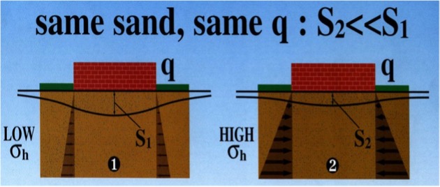
When the dilatometer blade is pushed into the soil, the geometry of the blade causes minimal volumetric and shear strain to the soil.  In contrast, when the cone penetrometer is pushed or standard penetration test split spoon is driven into the soil, their circular geometry causes significantly more volumetric and shear strain to the soil.  Figure 1 illustrates the differences in the straining of the soil due to their different geometries (Baligh, Scott, 1975).  Marchetti (1998) shows that arching occurs when pushing a circular probe, while the dilatometer blade knifes into the soil with little arching effects, resulting in more accurate stress history measurements (Figure 2).

Less disturbance pushing the DMT blade than conical probe

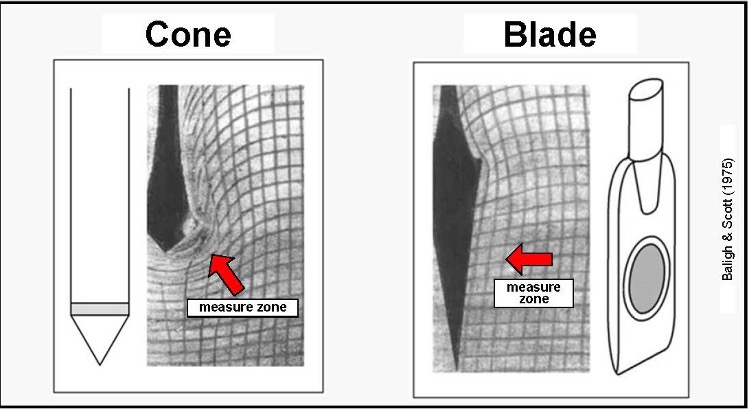
Figure 1:Less disturbance pushing the DMT blade than conical probe (CPT or SPT)

Arching Effect

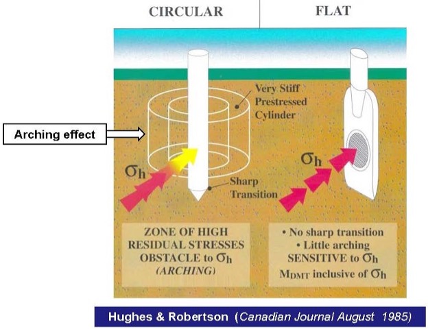
Figure 2: Significant arching caused by pushing conical probe versus little arching by pushing sharpened blade that knifes into the soil

 The dilatometer blade has a cross-sectional area of about 14 cm2. A direct push rig with about 15 tons (13,000 kgf) of thrust can advance it into soil with an N60-value of about 40 blows per foot, while a heavy drill rig with about 5 tons (4,000 kgf) of thrust can advance it into soil with an N60-value of about 25 blows per foot. Tests can be successfully performed in all penetrable soils, including clay, silt, and sand. If the soil contains a significant amount of gravel, however, point contacts against the membrane instead of a continuous medium may cause inaccurate results. Furthermore, gravel will often tear a hole in the membrane. The engineer can identify tests in soil containing gravel as they have low “A” readings from point contacts resulting in high material indices and low pre-consolidation pressure correlations. Furthermore, when pushing the dilatometer blade into these materials, the soil makes a crunching sound as the gravel fractures—not music to the engineer’s ears. While ASTM allows the DMT blade to be driven into the soil, we believe that this method causes additional disturbance to the soil and discourage this method.

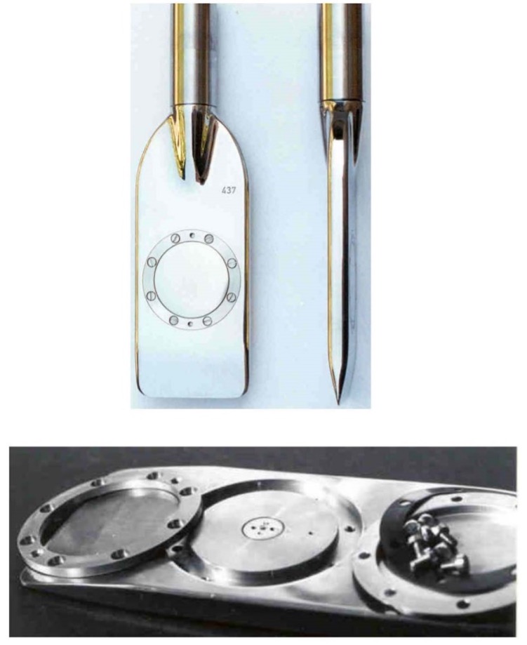
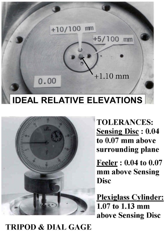
Figure 3 shows a dilatometer blade and a dilatometer blade with its membrane removed; Figure 4 shows the tolerance for the sensing disk, feeler (lift-off point for the “A” reading), and the fully extended Plexiglas cylinder (fully expanded position of the membrane for the “B” reading); Figure 5 shows the working principle for the “A” and “B” readings; and Figure 6 shows the general set-up for the dilatometer test.


Assembled dilatometer blade and dilatometer blade with membrane removed
Tolerances for sensing disk, feeler, and Plexiglas cylinder

Figure 3 (left): Assembled dilatometer blade and dilatometer blade with membrane removed
Figure 4 (right): Tolerances for sensing disk, feeler, and Plexiglas cylinder

Working Principle of Dilatometer
General layout of the dilatometer test

Figure 5 (left): Working Principle of Dilatometer
Figure 6 (right): General layout of the dilatometer test

Membranes have thicknesses of either 0.20, 0.25 or 0.30 mm. To confirm that no significant changes occur in the membrane calibrations (resistance in air), each new membrane must be exercised or stretched using pressures of 6 bars or more until their calibrations become stable. Typically, new 0.20 and 0.25 membranes have ΔA = 0.15 and ΔB = 0.45, while new 0.30 membranes have ΔA = 0.25 and ΔB = 0.80 calibrations. The 0.25 membranes work best for soil without gravel or debris as their before and after calibrations do not change much, while the more robust 0.30 membranes work best where gravel or debris occurs or on barge projects, where the delay costs to change a membrane are high. The membrane rests between the “A” and “B” readings and has no electrical continuity. A syringe applies a vacuum to the blade until the membrane contacts the blade and electrical continuity occurs. The engineer slowly releases the vacuum until the electrical continuity stops and he/she records that vacuum value as the ΔA reading. Although ΔA has a negative value of pressure, the engineer records this value as a positive value because the data processing software expects a positive number for its formulae. The engineer then applies pressure through the syringe to the blade until it moves the membrane to its fully expanded position (~1.10 mm) and the electrical signal activates. He/she records this pressure as the ΔB calibration measurement. Before and after each sounding, the engineer performs membrane calibrations at least three times or until he/she has obtained values ±0.01 bar. The engineer averages the before and after calibrations, and rounds down to the nearest 0.01 bar. (Marchetti, 1999)

Control Unit:  The control unit takes nitrogen from the pressurized tank and sends that pressure through a pneumatic/electrical cable to the dilatometer blade’s membrane and measures the pressure needed to inflate it.  The engineer should inflate the membrane slowly when the pressure approaches either the “A” (lift-off), “B” (fully-expanded) or optional “C” (recontact) dilatometer readings so that the pressure at the control unit equals the pressure in the dilatometer blade/membrane.  The pneumatic/electrical cable has a single wire that senses electric continuity of the membrane and connects to the underside of the sensing disk beneath the center of the membrane (Figures 7a-d).  A ground wire connects the control unit to the rods/blade and completes the electrical circuit.  When working over water, the engineer can simply put the grounding wire in the water to make continuity.

The original style control unit (Figure 8a) and an updated version (2015) that includes pressure transducer (Figure 8b) has two analog gauges-a low pressure gauge (-1 to 10 bars) and a high-pressure gauge (0 to 60 bars).  At approximately 9.5 bars a gauge minder switch discontinues pressurizing the low-pressure gauge to protect it from overextending and becoming damaged.  For pressures less than ~9.5 bars, the engineer measures the pressure with the more accurate low-pressure gauge to the nearest 0.01 bars.  Above 9.5 bars, he/she measures the pressure with the high-pressure gauge to the nearest 0.05 bars.  The engineer reads directly over the needle and uses the mirror under the needle to avoid parallax. 

Pneumatic-electrical cables
Throat detail
Male Connector
Female Connector

Figures 7a-d: Pneumatic-electrical cables; Throat detail; Male Connector; Female Connector 

Original style control unit

Figure 8a: Original style control unit

Updated control unit-transducer/seismic

Figure 8b: Updated control unit-transducer/seismic

In 2006, a computer using an “add-on” box that connects to the side of the original control unit contained a pressure transducer to make more accurate measurements (Figure 9). The “add-on” box eliminates the human gauge reading error and updates the acquisition system for shear wave measurements from the seismic module.

In 2020, the “Medusa” automatic dilatometer probe was manufactured (we own serial numbers 01 and 02). Basically, the “Medusa” has its control unit downhole in a module just above the blade. This system has an electrical motor that moves a miniature piston that pressurizes vegetable oil that either pushes or retracts the membrane (Figure 10). It has a pressure transducer that makes the measurements and transmits them via a data cable to the computer at the surface. Because the “Medusa” knows how far the piston needs to extend for each reading, it makes those readings accurately at ~15 second intervals, based on the electrical continuity as with the other control units. The “Medusa” eliminates the time lag for the pressure at the control unit to equal the pressure at the membrane. It measures the “A” reading either while the blade stops for a complete “A” dissipation test or while the blade pushes into the soil for a continuous “A” reading or horizontal stress profile.

“Add-on” Box

Figure 9: “Add-on” Box

Medusa Automatic DMT

Figure 10: Medusa Automatic DMT

Performing Dilatometer Tests:

Thrust measured at surface compared favorably with downhole
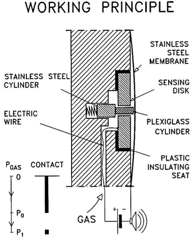
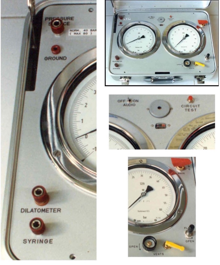
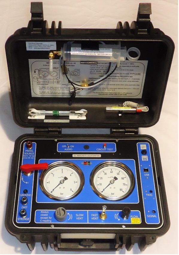
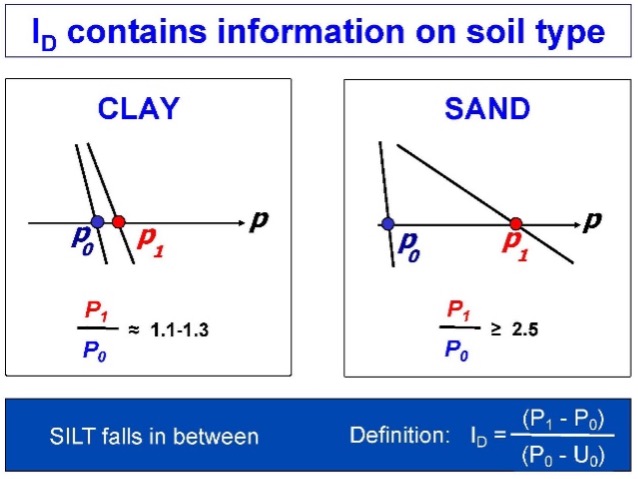
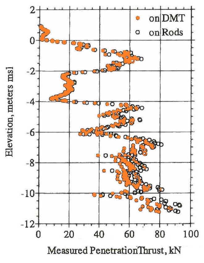
After pushing the dilatometer blade at the ASTM constant rate of 2 cm/second to the test depth, the engineer inflates the membrane outward, first measuring the pressure where the membrane lifts off from the blade (“A” reading) and the pressure where the membrane is fully expanded (1.1 mm away from the blade) (“B” reading). The surrounding soil usually collapses the 60-mm-diameter stainless steel membrane flush against the blade during the penetration, providing electrical continuity for the “A” reading. (In very weak soils, the engineer may need to apply a vacuum to make the membrane contact the blade prior to pushing.) The engineer should measure the thrust needed to advance the blade to the test depth. Bullock (2015) shows that thrust measurements made at the surface equaled measurements made at the friction reducer just above the blade if the soundings were less than 12 m (40 feet) (Figure 11). Calculation of the angle of internal friction, lateral stress coefficient at rest, and pre-consolidation pressure in cohesionless soil require thrust measurements. Before starting the DMT test, the engineer can compare the thrust measurement with previous thrust data and their corresponding dilatometer “A” and “B” readings, to predict what the dilatometer “A” and “B” readings may likely be. The ratio of “B”/“A” stays approximately the same for the same soil type. For cohesive soil that ratio approximates 1.5, while for cohesionless soil that ratio approximates 3. After measuring the “A” reading, and if the thrust is similar to the previous value, the engineer can assume that the soil type and its “B”/“A” ratio remain the same. The engineer can now make a good estimate of the “B” reading. The engineer should inflate the membrane more slowly as the pressures approach predicted “A” and “B” values, measuring those values more accurately.

The engineer should perform dilatometer tests at 20 cm depth intervals, conveniently working out to 5tests/meter long rod. Where thrust measures less than 500 kgf, which generally indicates a very soft soil, the engineer should reduce the test depth interval to 10 centimeters to provide more data for design in these critical soils.

Figure 11: Thrust measured at surface compared favorably with downhole

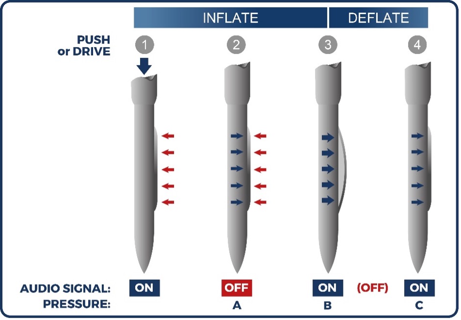
Below the groundwater table, the engineer can deflate the membrane and measure the pressure (“C” reading) where the deflated membrane recontacts the blade. Below the groundwater table, the “C” reading measures the hydrostatic groundwater pressure in a cohesionless soil or excess pore water pressures in a cohesive soil (Figure 12, Schmertmann and Crapps, 1988). In cohesive soil, if the engineer measures either “A” or “C” readings versus elapsed time, he/she can compute the time rate of consolidation as the pore pressures dissipate. Figure 13 shows the dilatometer test sequence.
P2 pore water pressure measurements versus depth

Figure 12: P2 pore water pressure measurements versus depth


Dilatometer test sequence

Figure 13: Dilatometer test sequence


Pore Pressure Dissipation Tests

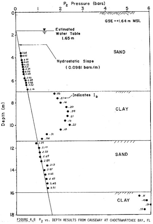
As the dilatometer blade pushes into the soil, it displaces the soil and pore water. In cohesive soil, pore pressures build up because the water cannot travel away from the displaced zone quickly enough. But as it travels away, the pressure decrease. We can measure the pore pressure dissipation or decay over time either 1) by creating a cavity from a dilatometer test and monitoring the decease in pressure versus elapsed time or 2) repeatly inflating the membrane at the lift-off position (A reading).

Example of “C“ Reading Pore Pressure Dissipation Test
The membrane expands to 1.1 mm to obtain the fully-expanded or B reading, and when it is deflated a cavity filled with pressurized water forms. The engineer can measure the water pressure decay by either moving the membrane from slightly expanded to closed position (“C“ dissipation test) or moving the membrane from the closed position to the lift-off position (“A2“ dissipation test). The elapsed time clock starts the instant that the dilatometer blade reaches the test depth. Eventually the cavity collapses from the cohesive soil swelling and the test ends as observed when the pressure measurements increase. Figure 14 presents an example of a “C“ dissipation test and the calculations for the time rate of consolidation and coefficient of permeability.

Figure 14: Example of “C“ Reading Pore Pressure Dissipation Test

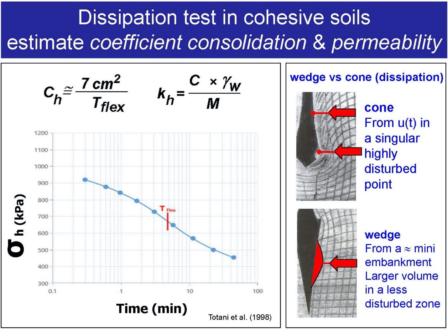
After pushing the dilatometer blade to the test depth, the engineer can repeatedly make the lift-off or A reading. Both the soil and excess pore water apply the resisting pressure. By plotting these measurements versus log of elapsed time, the engineer can find the flexure point on the curve, Tflex. The automated Medusa dilatometer system collects the “A“ measurements frequently and accurately to give the engineer high quality curves (Figure 15). Totani (1998) calculates the time rate of consoldiation and coefficient of permeability using the below formulas:

ch = 7 cm2/Tflex
kh = (chw)/M

“A“ Dissipation Test made with Medusa Dilatometer System

Figure 15: “A“ Dissipation Test made with Medusa Dilatometer System

After completing the dilatometer test sounding, the engineer extracts the rods and dilatometer blade from the ground, inspects the dilatometer blade, calibrates the dilatometer membrane, and can now continue to the next dilatometer test sounding.

Data Reduction:

The engineer corrects dilatometer “A”, “B”, and “C“ readings for the membrane stiffness in air, “ΔA” and “ΔB”, to get “P0”, “P1”, and “P2” values. The “P0”, “P1”, and “P2” values then compute the intermeadiate dilatometer indices, ID (Material Index), KD (Horizontal Stress Index), ED (Dilatometer Modulus) and UD (Pore Pressure Index). These multiple independent indices converge with accurate correlation equations to desired soil properties. Dr. Silvano Marchetti often described this method of creating correlation equations as “triangulation”–using two or more independent variables to hone in on a third dependent parameter. From the dilatometer test data, the engineer processes the data to obtain the following soil parameters (Figure 16):

  • Drained friction angle for cohesionless soil [φ’],
  • Undrained shear strength for cohesive soil [cu]
  • Total unit weight of soil [γt],
  • Coefficient of lateral earth pressure at rest [ko],
  • Preconsolidation pressure [pc], and
  • Over-consolidation ratio [OCR]
Marchetti (1980) equations

Figure 16: Marchetti (1980) equations


As shown numerically in the rectangular boxes on the Figure 16 chart, the unit weight increases as the dilatometer modulus, ED, increases. Cohesionless soil has a high ID, while cohesive soil has a low ID. Figure 17 illustrates the difference between identifying cohesive and cohesionless soils.

Figure 17: Differences identifying clays and sands

We use Windows DMT (WinDMT) computer program to process the field data. Figure 18 presents the legend for the output from WinDMT.

WinDMT Output Legend

Figure 18: WinDMT Output Legend

Figure 19 shows an example of the corrected dilatometer pressure readings for membrane calibrations and identifying the soil behavior type. 

Example Dilatometer Test Results

Figure 19: Example Dilatometer Test Results

Shear Strength: The engineer can complete a dilatometer test in one to two minutes. Soil with an ID < 0.6 test as undrained soil, while soil with an ID > 1.2 test as drained soil. Soil with an ID > 0.6 and < 1.2 test as partially drained soil. Either the undrained shear strength or the angle of internal friction correlations for soil tested as partially drained have uncertainty and error. Soil samples can provide the engineer with interpretation guidance. Sometimes, highly over-consolidated clay can have an ID between 0.6 and 0.9 and undrained shear strength correlations make good predictions. Sometimes, sandy residual soil with mica can have an ID between 0.9 and 1.2 and the drained angle of internal friction correlations make good predictions. For cohesionless soil, Marchetti’s correlation for the angle of internal friction provides a lower-bound and too conservative value. From theory for penetration of a rigid wedge developed by Durgunoglu and Mitchell (1973) for the Apollo mission to the moon, Schmertmann (1986) used elastic half-space theory with thrust measurements and the horizontal stress from KD, to accurately calculate the plane strain angle of internal friction. We only use this method because of its accuracy. Schmertmann suggests computing the triaxial angle of internal friction using the following:

φtxlps  for  φps <32°
φtxl = 32° + 2/3 * (φps – 32)  for  φps > 32°

For cohesive soil, Marchetti (1980) presented the below correlation for undrained shear strength:

Su = 0.22 * σvo’ * (0.5 * KD)1.25

Lutenegger (2006) presented the following correlation for undrained shear strength based on a cavity expansion model using the “P0” and “P2” readings:

Su = (P0 -P2)/2.65

Marchetti’s correlation provides an average value when compared to other type of tests as shown below at sites worldwide (Figures 20a-f):

Cu in Tokyo Bay Clay
Cu at Skeena Ontario Canada
Dilatometer-test-figure-20c
Dilatometer-test-figure-20d
Cu in 2 Malaysian Clays
Cu in Recife Clay - Brazil

Figures 20a-f: Marchetti Undrained Strength Comparisons from Sites Worldwide

For very soft clays in settling ponds for phosphate spoils in Florida, Bloomquist found the undrained shear strength from DMT compared quite well with vane shear tests as shown right (Figure 21).

The KD horizontal stress index provides a critical numerical parameter for stress history of the soil that other in-situ tests do not provide (Figures 22 and 23).

Figure 21: Comparison of undrained shear strength between DMT and VST in very soft clays

For very soft clays in settling ponds for phosphate spoils in Florida, Bloomquist found the undrained shear strength from DMT compared quite well with vane shear tests as shown right (Figure 21).

The KD horizontal stress index provides a critical numerical parameter for stress history of the soil that other in-situ tests do not provide (Figures 22 and 23).


Importance of KD.
Comparison of undrained shear strength between DMT and VST in very soft clays

Figure 21: Comparison of undrained shear strength between DMT and VST in very soft clays

Importance of KD.

Figures 22 and 23: Importance of KD.

Lateral Earth Pressure at Rest Coefficient, ko:  For clay and silt (ID < 1.2), Marchetti (1980) correlation predicts ko value reasonably well (Figure 24).  His formula follows:

ko = (KD/1.5)0.47 – 0.6   (ID < 1.2)

From large chamber testing of sand, Schmertmann (1983) found that Marchetti (1980) formula did not predict ko for sand and developed the below formula using both KD and φ’ax (Figure 25).

ko = 40 + 23 KD -86KD(1-sinφax) + 152(1-sinφax) -717(1-sinφax)2        (ID > 1.2)

192 – 717(1-sinφ’ax)

KD correlation with ko for ID < 1.2
KD correlation with ko for ID > 1.2

Figure 24: KD correlation with ko for ID < 1.2    Figure 25: KD correlation with ko for ID > 1.2

Figure 26: presents an example plot of dilatometer correlated shear strength parameters.

DMT Shear Strength Example

Figure 26: DMT Shear Strength Example

Deformation Properties: The dilatometer test statically deforms the soil straining it to intermediate levels compatible with strains that structures or embankments generate.  On the other hand, penetration tests (CPT and SPT) strain the soil to failure making those correlations with deformation modulus inaccurate (Figure 27).  Logically and intuitively, the engineer knows deformation tests better predict the soil’ stiffness than penetration tests that fail the soil.

Elastic half-space theory used to compute ED

Figure 27: DMT strains the soil to an intermediate level like buildings or embankments

Figure 28: Elastic half-space theory used to compute ED

The dilatometer modulus, ED, acts as an intermediate parameter (the engineer should not use ED in any design calculations) and requires correlation equations based on ID and KD to get the constrained deformation modulus, M.  M equals the tangential slope from a consolidation test plotted arithmetically as vertical strain versus applied pressure at the existing vertical effective stress (Figure 29). On Figure 30 Failmezger and Bullock (2004) shows how favorably DMT M values compare with laboratory consolidation tests for alluvial and residual soils.  Figure 31 shows favorable comparisons of constrained deformation moduli for soil in Norway and Tokyo between DMT and laboratory consolidation test data.

Computing Constrained Deformation Modulus from Lab Consolidation Tests
DMT Favorable Comparisons with Lab Consolidation Tests (close to 1:1 line)

Figure 29: Computing Constrained Deformation Modulus from Lab Consolidation Tests

Figure 30: DMT Favorable Comparisons with Lab Consolidation Tests (close to 1:1 line)

Figure 31: DMT and Consolidation Tests Comparisons for Constrained Deformation Moduli in Norway and Tokyo

Over-consolidation Ratio: For cohesive soil with an ID < 1.2, Marchetti (1980) computes the OCR with the following equation:

OCR = (0.5 * KD)1.56        For ID < 1.2

For cohesionless soil, Schmertmann slightly modified Mayne and Kulhawy (1982) formula to have a better correlation with large chamber test data as follows:

OCR = [ko/(1 – sinφ’ax)](1- 0.8 * sinφ’ax)                                  

                              For ID > 1.2

DMT and Consolidation Tests Comparisons for Constrained Deformation Moduli in Norway and Tokyo

Figure 32 presents an example of modulus and preconsolidation pressures for a DMT soundings.

Example of Deformation Modulus and Preconsolidation Pressure

Figure 32: Example of Deformation Modulus and Preconsolidation Pressure

Schmertmann and Crapps (1988) estimate the accuracy of dilatometer correlations of geotechnical soil properties by comparing with superior measurements (Figure 33).

Figure 33: Comparison of Dilatometer Correlations with Superior Tests (PennDOT Manual)

Settlement Calculations:

Because the dilatometer test statically deforms the soil at intermediate strain level similar to a building or embankment, its data accurately predict the amount of settlement that will likely occur.  Schmertmann (1986) presents two methods to compute settlement, the 1) ordinary and 2) special methods.  The ordinary method uses the following formula based Janbu’s method:

            S = Δσv * H / M, where

            S = predicted settlement,

            Δσv = increase in vertical stress,

            H = the layer thickness, and

            M = the constrained deformation modulus.

The engineer cannot average M values to compute settlement because M is a denominator term (would result in a mathematical error).  The engineer should use each test and its depth interval as a separate layer in the above formula and then sum the delta settlements to compute the total settlement.  The special method accounts for the soil’s preconsolidation pressure in its settlement calculations.  Excel spreadsheets that make settlement calculations for the ordinary and special methods have the following links (Boussinesq stress distribution, Harr stress distribution).  The Boussinesq stress distribution computes the increase in vertical stress assuming the soil behaves as an elastic material.  The Boussinesq distribution does not consider the material properties of the soil.  A vertical load placed on soil causes the soil particles to move downward and closer together as water exits the void spaces, move laterally out of the way or crush into smaller pieces occupying less space.  The Harr stress distribution follows random path probability theory (modeled similarly to water dripping from a leaky faucet) and uses the bell-shaped normal probability distribution.  His method includes the coefficient of lateral stress, which interestingly the dilatometer predicts.

Δσz = P/(2πkoz2) * exp[-(x2 +y2)/2koz2

Δσx = x2/z2 * Δσz

Δσy = y2/z2 * Δσz

For stress directly beneath the center of the force, the formula simplifies to:

Δσz = P/(2πkoz2),

Where Δσz is the most probable value of vertical stress increase,

            Δσx is the most probable value of horizontal stress increase in the x direction,

            Δσy is the most probable value of horizontal stress increase in the y direction,

            ko is the coefficient of lateral stress at rest, and

            P is the applied load.

For uniform bearing pressures, Failmezger (2022—to be published) shows that Boussinesq method equates to approximately a ko = 0.4 for Harr’s method as shown on Figures 34a (circular), b (square) and c (L = 10B rectangular) Stress bulbs and factors for Boussinesq and Harr ko for circular, L=B, L=2B, L=5B and L=10B

Stress Factor
Stress Factor
Figure 34: Comparison of Stress Factors beneath Center of Circular, Square and Rectangular Footing for Boussinesq and Harr k0 Methods

Dilatometer tests with thrust measurements provide reasonable values of k0 for the analyses. Because k0 values can have outliers due to cementation and gravel particles, the engineer should use the median rather than the mean or average value for k0 for computing the stress distribution with the Harr method. Marchetti (1998) illustrates the importance of horizontal stress in Figure 35.

Figure 35: Importance of Horizontal Stress

Schmertmann (1986) and Hayes (1986) made class “A” (first made prediction, then made measurement) settlement predictions using Schmertmann’s method for 22 projects.  They accurately predicted settlement as they closely follow the 1:1 line shown as Figure 36.  Their average ratio of predicted settlement from dilatometer analysis versus actual measured long-term settlement equaled 1.07 with a standard deviation of 0.22. 

Figure 36: Schmertmann and Hayes settlement predictions versus measured settlement

Schmertmann and Hayes settlement predictions versus measured settlement

Monaco 2006, most predictions based on Schmertmann’s 1986 method, and Godlewski 2018, most predictions based on finite element analyses, show similar accuracy for settlement predictions as Figures 37 and 38.

Monaco settlement predictions

Figure 37: Monaco settlement predictions

Godlewski settlement predictions

Figure 38: Godlewski settlement predictions

Failmezger (2021) shows 130 projects where geotechnical design using dilatometer tests saved $25,000,000 instead of using design based on SPT (Table 1). 

Table 1 Cost savings by using DMT to redesign the foundation system

PROJECT NAME

COST SAVINGS WITH DMT REDESIGN OF FOUNDATION SYSTEM

Westminister Village$100,000
Ocean Landing Shopping Center$750,000
Old Town Crescent$150,000
Fox Run Village$100,000
Monarch Landing$150,000
MD Live!$2,000,000
Towson Circle$200,000
Retirement Community, Glen Mills, PA$150,000
Xfinity Live!$500,000
Obery Court$200,000
Residences at Rivermarsh$100,000
Residences at River Place$80,000
Ocean Pines$200,000
Four Seasons$100,000
912 King Street-116 S Henry Street Mixed Use$500,000
Dumfries Town Square$200,000
Seacobeck Hall—Mary Washington University$500,000
Motown$150,000
Richmond Area Collegiate Science Building$85,000
Richmond Area Collegiate Research Building$150,000
Food Processing Addition and Tank Farm$100,000
13th and U Street$100,000
55 M Street$150,000
Alexan Dunn Loring Development$250,000
Association of Manufacturing Technology Building$150,000
Excelsior Parc Development$100,000
Glenmont WMATA$150,000
Halley Rise $150,000
Howard Hughes HHMI Expansion$100,000
I-64 Widening$500,000
JHU-NIH-NCI$150,000
Mark Center Plaza Building 5$150,000
Mosaic Parcel CE$100,000
National Gateway Land Bay “E” West$250,000
Potomac Yard Bay D$150,000
Ripley Street Development$100,000
Rock Spring Centre$250,000
Route 7 over Dulles Toll Road$150,000
Route 7 Widening$350,000
Tysons Archstone$150,000
Tysons Central$250,000
Upper Rock Blocks G & H$100,000
West Falls Church WMATA$150,000
McWane Hall—Lynchburg College$100,000
Brooktrout$50,000
Mecklenburg Schools$100,000
Abingdon Elementary School$225,000
Abingdon Heights$400,000
Fauquier High School$250,000
Prince William Commons$400,000
PWCPS Administration Bldg$225,000
Warrenton Aquatic & Recreation Facility$250,000
Washington Center$350,000
WMATA White Flint Parking Garage$625,000
3800 Glenwood$350,000
Homewood Suites$150,000
Johnson County WWTP$1,000,000
1011 M Street$200,000
14th and W Street$200,000
1600 7th Street$50,000
300 8th Street$125,000
A-1 Glass$100,000
B-CC High School$350,000
Carlisle$200,000
Fairfax Blvd Center$100,000
Forest Oak Middle School$100,000
Grimke$150,000
Kilmer Place$50,000
Liberty Tank$100,000
Sumner Suites$125,000
Windsor$50,000
Wood Middle School$75,000
Wootton$75,000
14th and P Street$150,000
Culpepper Farmers’ Coop$50,000
Indian Head Water Tanks$75,000
Portals Phase 3$175,000
Thomas Jefferson Library$75,000
Avalon Mosaic Parcel H$800,000
Cabin John Middle School$200,000
Navy Federal Credit Union$100,000
Cambridge Village$150,000
Ben Oaks Water Tower$75,000
Apple Greene Water Tower$50,000
Oyster Bay Condos$100,000
North Beach Various Parcels$50,000
Fort Meade-DINFOS$200,000
Fort Meade-Building #8605$50,000
Fort McNair-Building #48$250,000
535 Broadwater Road$50,000
15 Judith Sound Circle$8,000
318 Ironside Circle$50,000
Courthouse Professional Building$60,000
Dahlgren Hotel$75,000
Doc Stone MOB$40,000
Hamptons at Hunton Park$60,000
Kaeser Compressors Warehouse Expansion$80,000
New Post Site$50,000
Oakwood Estates$85,000
Sophia and Hanover Streets$40,000
1112 First Street Hotel$250,000
Courthouse Village Bridge$250,000
Arbor House$100,000
William Square Hotel$250,000
James Madison University—Phillips Hall$150,000
1336 H Street$80,000
Aspire at Lee’s Hill$35,000
DHL Stafford$25,000
Mapledale Storage$50,000
Pruitt Laburnum Property$80,000
Wilson YMCA$250,000
Multi-Story Residential—Richmond, Virginia$50,000
Industrial Complex—Hanover, Virginia$250,000
Tank Farm—Cumberland, VA$30,000
Industrial Facility—Eastern NC$100,000
Industrial Facility—King William, Virginia$50,000
Industrial Facility—King William, Virginia$100,000
Multi-Story Office and Parking—Richmond, Virginia$75,000
3700 National$250,000
Andrews Air Force Base$100,000
Potomac Yard Land Bay “F”$250,000
Waterfront Station$150,000
Rustburg Middle School$200,00
Mechlenburg Middle/High Schools$200,000
Annapolis Junction Building 3$250,000
Annapolis Junction Building 4$250,000
116S Henry Street$750,000
QTS$500,000
Reston Crescent$90,000

Total Cost Savings

$25,053,000

Lateral Load Capacity of Deep Foundations:

Dr. Silvano Marchetti originally developed the dilatometer to predict the lateral load capacity of piles.  Because the DMT pushes the soil horizontally, it models a pile pushing against soil.  Marchetti, et al., 1991 modeled the lateral capacity of a pile against cohesive soil and Robertson, et al., 1989 modeled the lateral capacity against both cohesive and cohesionless soils (Robertson Excel spreadsheet).  The engineer can determine accurate P-y curves and continuous P-y profiles from those methods and use them with numerical computer programs such as LPILE and COM624.  Figure 39 shows how well both methods predict lateral load capacity.

Figure 39: Accurate lateral capacity predictions with dilatometer tests

Accurate lateral capacity predictions with dilatometer tests

Ground Improvement Evaluations:

“Aged” soil has higher deformation modulus than recent compacted fill that has lower void ratio

For ground improvement projects, dilatometer tests evaluate the effectiveness of the improvement method by performing tests before, during and at completion of the improvement.

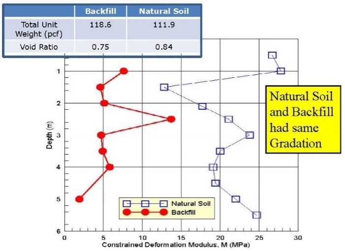
 Ground improvement techniques often increase lateral stresses, increase the shear strength and deformation modulus and decrease the void ratio.  An “ageing” process further increases the shear strength and stiffness (Schmertmann, 1991-Terzaghi Lecture).   “Aged” soil can have significantly higher deformation moduli even if its void ratio exceeds soil with the same gradation but recently compacted (Figure 40).  Because improved soils will have fairly heterogeneous properties, vertically and horizontally, many tests are needed to confirm that the soils have been adequately improved at all desired locations.

Figure 40: “Aged” soil has higher deformation modulus than recent compacted fill that has lower void ratio

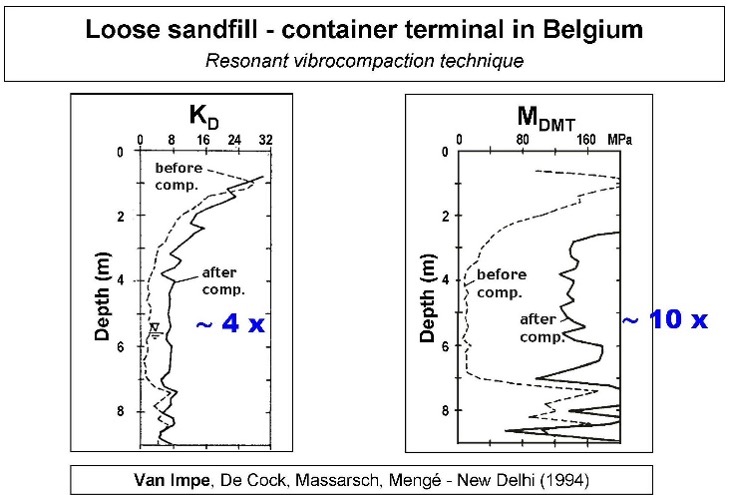
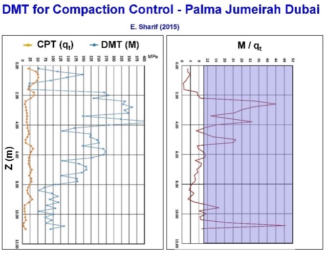
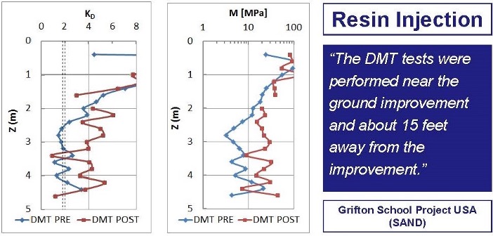
In-situ tests with high shear strain and disturbance effects measure ground improvement poorly because they damage soil structure.  Because the DMT accurately measures both the soil’s deformation modulus and the at rest lateral pressure with minimal ground disturbance, they provide an excellent choice to determine whether the soil has sufficiently improved.  As documented at the St. Johns River Power Plant near Jacksonville, Florida, the dilatometer M values more accurately evaluated soil improvement than relative density correlations based on electronic cone qc values. (Schmertmann, et al., 1986).   The dilatometer KD and M values have great sensitivity to prove ground improvement at three different sites (Figures 41 a-c).

Three sites showing dilatometer KD and M measuring ground improvement

Figure 41 a-c: Three sites showing dilatometer KD and M measuring ground improvement

Detecting Slip Surfaces in Over‐Consolidated Clays:

When a landslide develops through an over-consolidated clay, it remolds the soil during the slide, and then the soil returns to a normally consolidated state after the slide halts.  The dilatometer KD value for an over-consolidated clay significantly exceeds 2, while a normally consolidated clay has a KD approximately equal to 2 (Figure 42).  Totani (1997) explains in further detail how dilatometer tests can locate slip surfaces from landslides.  Figures 43 a-c identify documented slip surfaces at three sites.

Detecting slip failure surfaces using DMT KD

Figure 42: Detecting slip failure surfaces using DMT KD

Figures 43 a-c: Detecting Slip Surfaces using DMT KD at three sites

Seismic Tests:

Air hammer to generate horizontal seismic strike
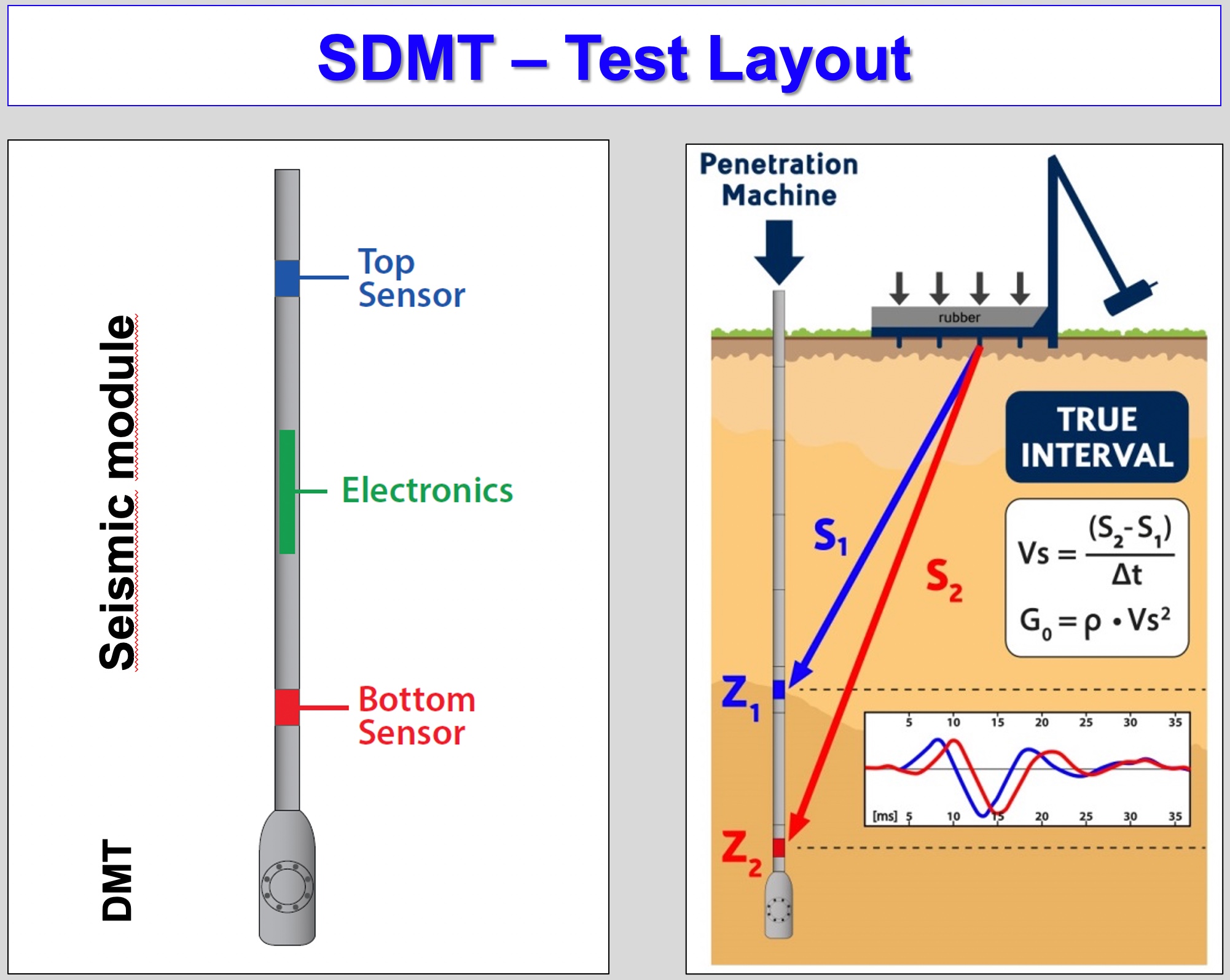
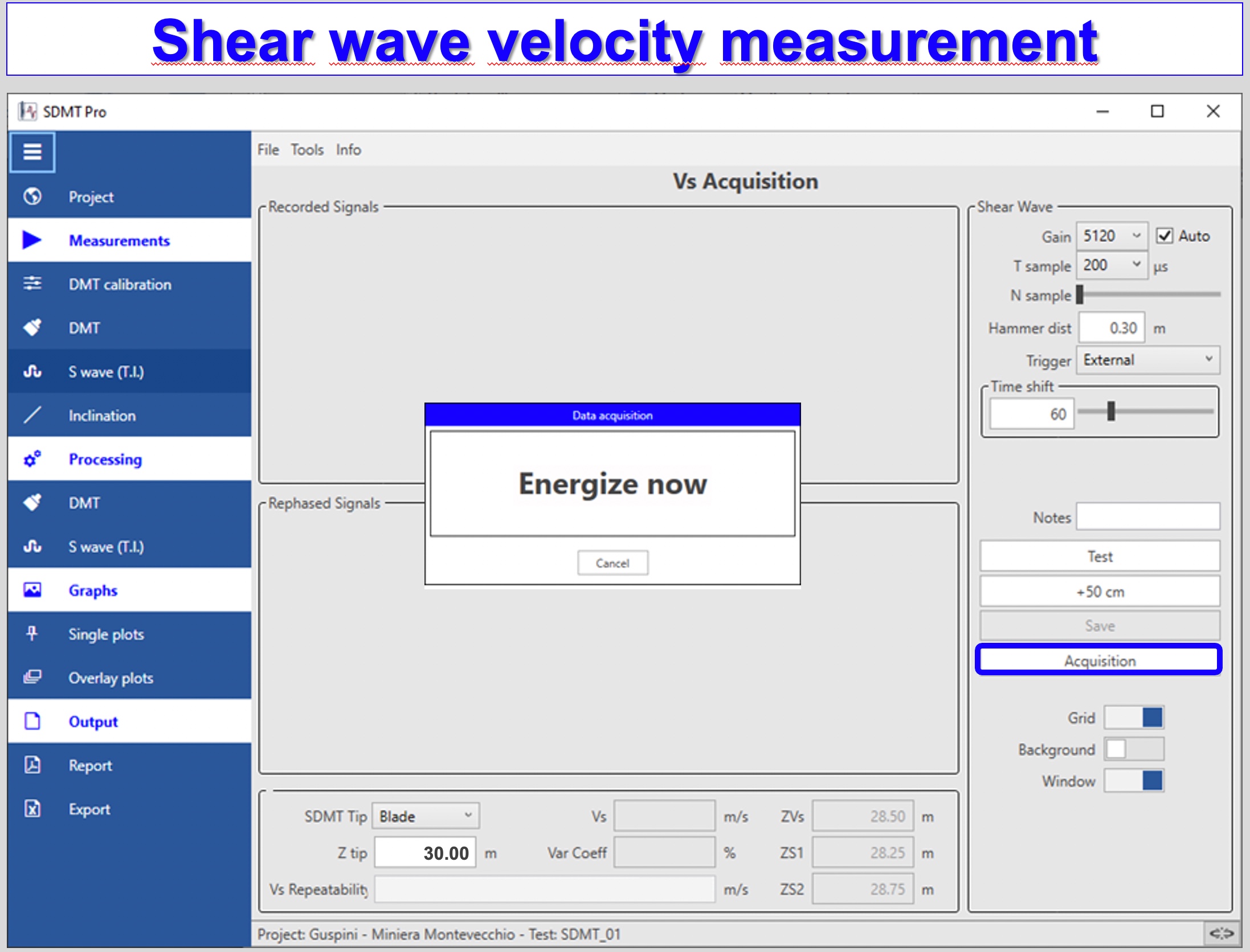
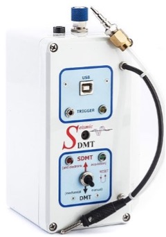
At the Second International Conference on the Flat Dilatometer in April 2006, the true interval seismic test was unveiled.  Two geophones spaced exactly 0.50 meters apart in a module located directly above the blade measure the seismic shear waves.  After a horizontal strike of a plate at the ground surface, a shear wave travels through the soil (Figure 44).  The upper geophone receives it first and then the lower geophone receives the same wave.  Both waves are recorded, digitally processed, and trans 
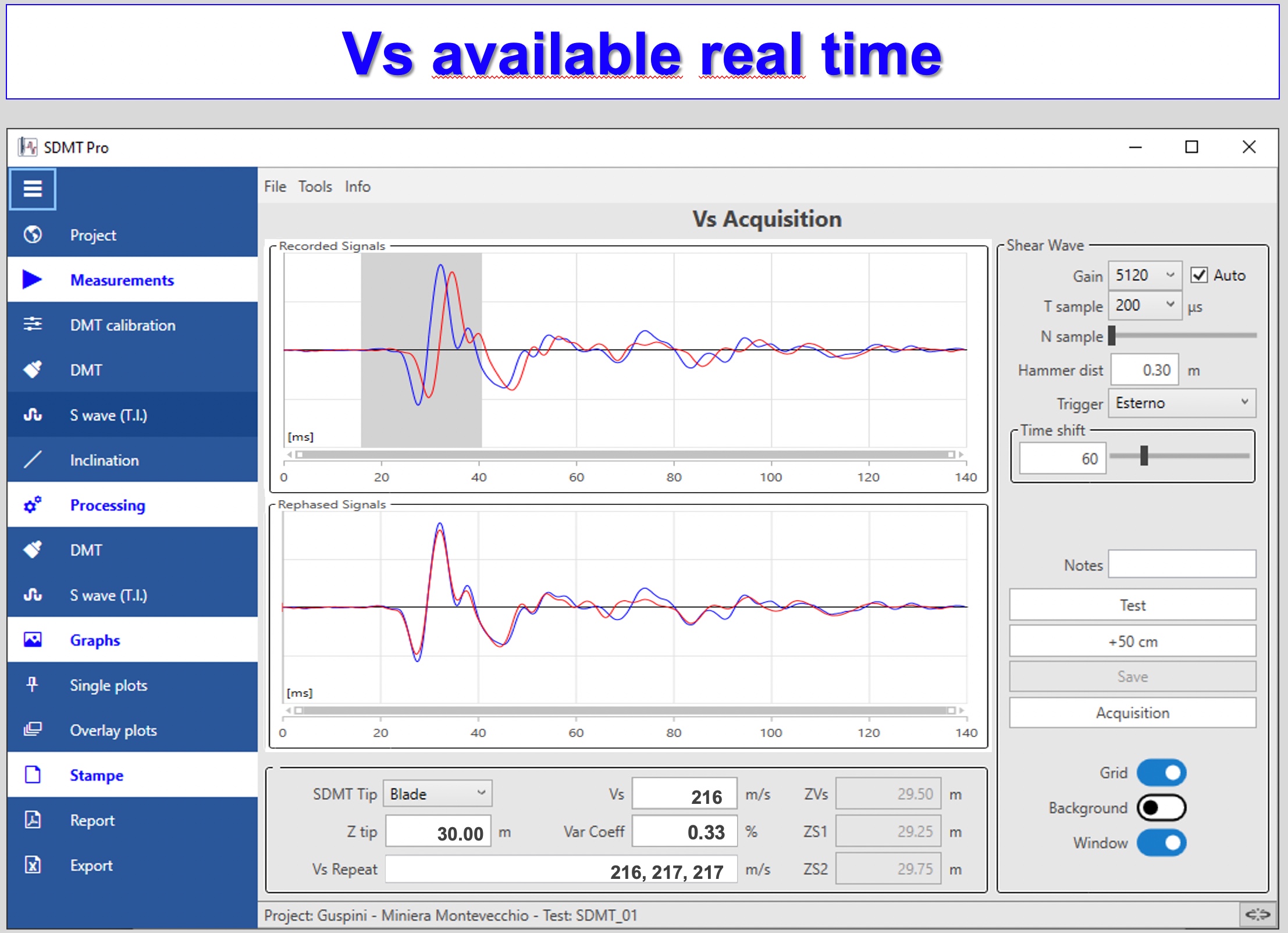
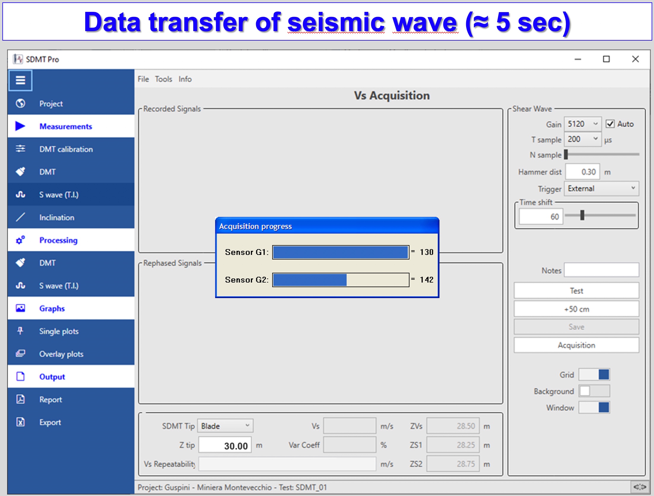
mitted serially through the single wire DMT cable to the computer at the surface.  The engineer shifts the second wave to the left by a delta time superimposing it on the first wave.  The shear wave velocity easily computes as the hypotenuse difference in the shear wave travel distances between the upper and lower geophones by this computed delta time.  At each test depth, the engineer repeats the seismic test at least three times, confirming similar shear wave velocities.  If he/she records any anomalies, he/she performs additional tests to verify the correct measurement.  Usually only three good strikes are needed, and the shear wave velocities agree within 1 foot/second.  Figures 45a-d show the seismic strike and the data acquisition computer screenshots.

Figure 44: Air hammer to generate horizontal seismic strike

Figures 45a-d: True Intervals Seismic Setup and Data Acquisition Screenshots

The shear modulus degrades with increasing shear strain.  With the seismic DMT test, the engineer obtains two data points on the degradation curves as follows:

            Gmax = ρ * Vs2

            Where Gmax = low strain shear modulus,

            ρ = mass density

            Vs = shear wave velocity

            GDMT =

            γDMT = 0.05 to 0.10%

Figures 46 shows how to create shear modulus degradation curves and Figure 46 shows examples of shear modulus degradation curves.

Example of Shear Modulus Degradation Curves

Figure 47: Example of Shear Modulus Degradation Curves

For liquefaction analyses, correlation charts shown as Figure 48 provides zones of liquefaction to the left side of the design line for KD and Vs.  Determining potential liquefactions using two separate design charts gives the engineer confidence in his/her design.  Figure 49 shows liquefaction analyses for a site.

Design charts for liquefaction

Figure 48: Design charts for liquefaction      

Example liquefaction analyses

Figure 49: Example liquefaction analyses