- Benefits of the Soil Pressuremeter Test
- Performing the Pressuremeter Test
- Processing the Pressuremeter Test Data
- Interpretation of Pressuremeter Test Results
- Judging the Quality of the Pressuremeter Test
- Shear Strength Parameters
- Design of Shallow Foundations
- Design of Deep Foundations
- Lateral Load Capacity for Deep Foundations
Soil Pressuremeter Test
Benefits of the Pressuremeter Test:
- Can be conveniently used with drilling equipment
- While tests can be done in soft clay or loose sands, the test is best used in dense sands, hard clays and weathered rock which cannot be tested with push equipment.
- An extensive database of load test results allows the geotechnical engineer to accurately design for shallow foundations and for lateral and vertical capacity of deep foundations.
- Can model a load test for shallow foundations and account for time dependent settlement

Figure 1: Foundations for the tallest buildings in world based on pressuremeter test data
Pressuremeter Test (PMT), ASTM D 4719: Louis Menard began his work with the pressuremeter test in 1954 while still a college student, studying first under Professor Kerisel in France, and later under Professor Ralph Peck at the University of Illinois. Menard improved and advanced a foundation test concept begun by Kogler in 1933, and then returned to France in 1957 where he started a company to build and use the PMT. He compiled a large data base of load tests and companion pressuremeter tests to refine his empirical design formulas and persuade other engineers to use the PMT. To show his confidence and encourage acceptance of the test, Menard guaranteed foundation designs based on the PMT with $10,000,000 of professional liability insurance from Lloyds of London (Hartmann, 2008). Laboratoire Central des Ponts et Chaussées (LCPC) has performed numerous shallow footing, vertical and lateral deep foundation load tests and companion pressuremeter tests verifying the accuracy of design methods based on pressuremeter tests. Mr. Clyde Baker, who has designed half of the world’s largest buildings relies on pressuremeter tests for his designs (Figure 1). APAGEO (2018) updated the French interpretation and application of pressuremeter test results for foundation design. Philip, et. al. 2020 present a design method for retaining walls using finite element model with pressuremeter moduli values.
The engineer performs pressuremeter tests by either 1) self‐boring the pressuremeter to the test depth, 2) pre‐boring a hole with drilling equipment and lowering the pressuremeter to the test depth or 3) pushing a pressuremeter to the test depth. Using either the self‐boring or preboring method, the driller can create a test zone with minimal disturbance. When the pressuremeter probe pushes into the soil, significant disturbance to the soil can occur. Failmezger (2014) measured significantly different strengths and stiffnesses when comparing pre‐bored and pushed‐in pressuremeter tests in a sensitive over‐consolidated Miocene‐aged cohesive soil. The engineer should not use empirical design equations established for prebored pressuremeter tests for pushed‐in pressuremeter tests without modifying the correlation coefficients.
Ideally the pressuremeter test provides an axisymmetric, plane strain test (the horizontal plane), typically drained in cohesionless soils and undrained in cohesive soils. Early pressuremeter probes used guard cells inflated with air at their top and bottom to force the central measurement cell inflated with water to expand only in the lateral direction. Briaud (1989) [FHWA Manual] showed that the error in test results did not exceed 5% for single-cell probes, also known as mono-cell, versus tri-cell pressuremeter probes (Figure 2) with a length at least six times its diameter. Marcil (2021) compared pressuremeter test results from Texam monocell with either metal or vulcolan rings and Menard tricell probes in different stiffness calibration tubes. While the results compared favorably, he suggests a slight correction to get a pressuremeter Menard modulus from Texam probes. He found no difference in the limit pressures between the probes. We thank Dr. Jean-Louis Briaud, who provided many of the charts and tables. (Figure 3 shows Failmezger and Briaud at GeoCongress 2019—both looking good in their blue suits).
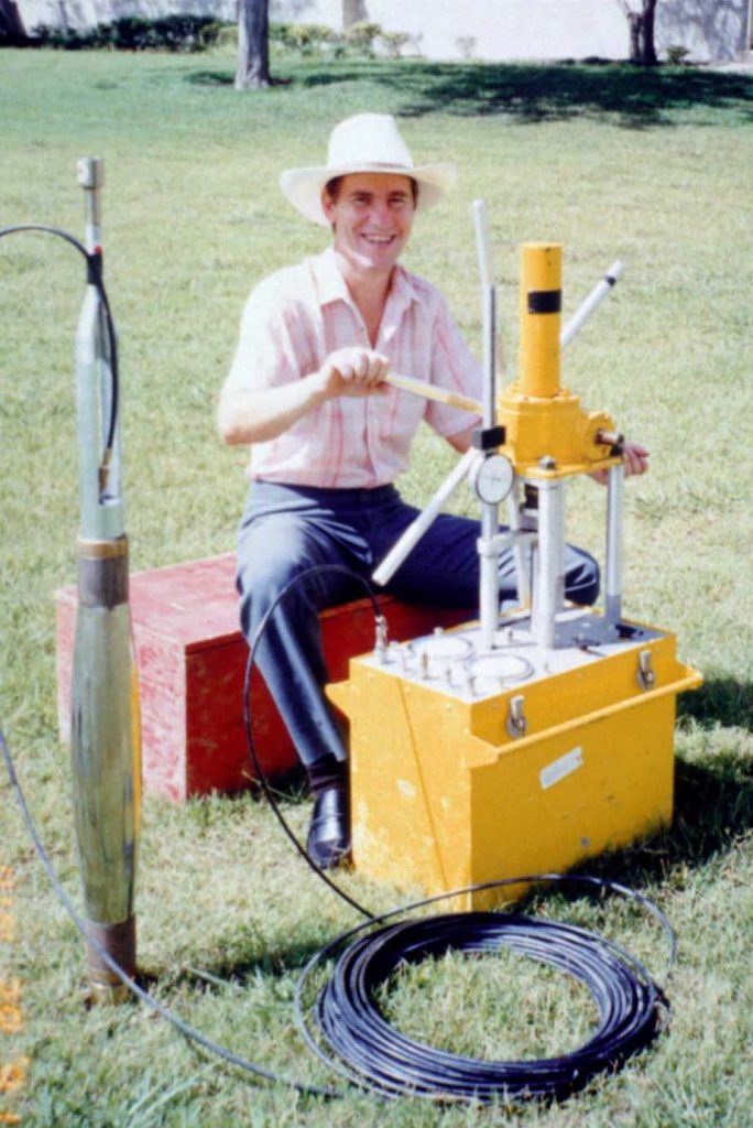
Figure 2: Dr. Jean‐Louis Briaud showing Texam pressuremeter

Figure 3: Briaud and Failmezger at GeoCongress 2019
Performing the Pressuremeter Test:
The engineer performs a pressuremeter test by inserting a calibrated pressuremeter probe into a carefully prepared borehole and inflating its flexible membrane in the lateral direction to a maximum radial strain of 40% depending on the probe design. He/she fills the control unit, tubing, and probe membrane with water, which is virtually incompressible, and measures the injected water for the volume and pressure for the test. The engineer can mix the water with ethanol glycol when temperatures are below freezing. He/she may expand the pressuremeter probe in equal pressure increments (stress-controlled test) or in equal volume increments (strain-controlled test), typically stopping the test when initial volume of the borehole diameter has doubled or more likely when the pressure becomes nearly asymptotic with increasing radial strain or volume. Because the engineer makes about 40 measurements with a strain-controlled test versus about 10 data points from a stress-controlled test, he/she will obtain a better-defined curve from strain-controlled tests.
The quality of the pressuremeter test measurements critically depends on the quality of the prepared test hole. The pressuremeter test simulates a high-quality laboratory triaxial test except it tests the sidewalls of a borehole instead of a high-quality undisturbed soil sample. The engineer should critically monitor the drilling of the borehole to assure that minimal disturbance occurs to the soil. After each test, he/she should discuss the hole quality with the driller and what adjustments the driller should make (if any) to the drilling technique to make a better-quality test hole.
On one major project, Failmezger performed pressuremeter tests, where the driller carefully prepared the borehole test zone using mud rotary methods, but for the second phase of explorations another testing firm performed pressuremeter tests instructing the driller to prepare the test zone by driving an over-sized split spoon. The design engineer called Failmezger and asked him why Failmezger’s pressuremeter tests showed the soil stiffness and strength was 4 times more than those values that the other testing firm reported. Failmezger replied “How did the other testing firm make the hole?” After the designer told Failmezger that they had driven an over-sized spilt spoon to make the test zone, he replied that they had completed disturbed the soil and only tested remolded soil. Afterwards the designer instructed the other testing firm to perform pressuremeter tests using mud rotary drilling techniques adjacent to a pressuremeter test borehole that Failmezger had previously done. Afterwards, the designer called Failmezger back and told him the new pressuremeter test results now compared favorably with those that Failmezger had performed earlier. Unfortunately driving an over-sized split spoon to make a pressuremeter test zone occurs far too often on the East coast of the United States. No engineer would consider performing triaxial tests using a sample from a SPT—why would any engineer consider designing based on pressuremeter tests from a borehole made by driving an over-sized SPT spoon?
We recommend the following hole preparation, testing, and calibration methods:
Hole Preparation:
- Above the pressuremeter test zone, the driller should make the hole about 4 inches (100 mm) in diameter with either 4 inch (102 mm) ID casing, 4.25 inch (108 mm) ID augers or 3-7/8 inch (98 mm) drill bit.
- For cohesionless soil the driller should use mud rotary drilling with a 3-1/16” (78 mm) diameter tri-cone bit with bottom discharge to make the test zone. For cohesive soil, the driller should use a 2-15/16 inch (75mm) diameter three winged bit with downward discharge. Figures 4a-b show drill bits used to make a high quality pressuremeter test hole.
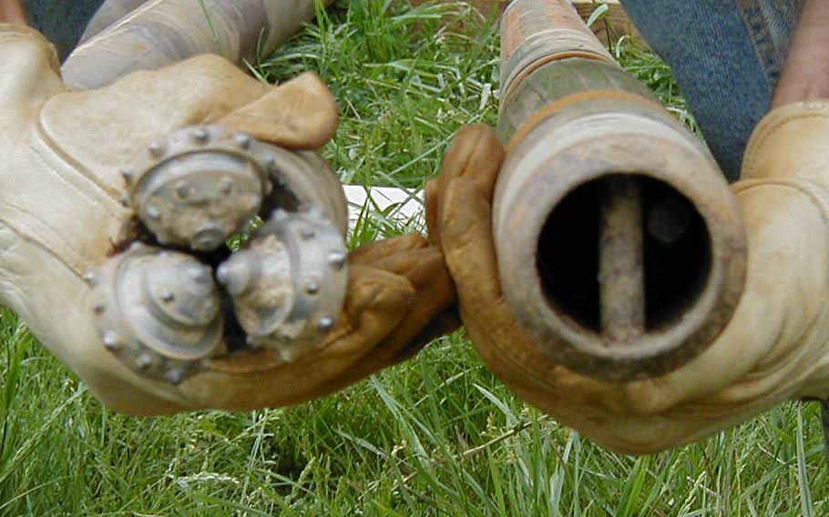
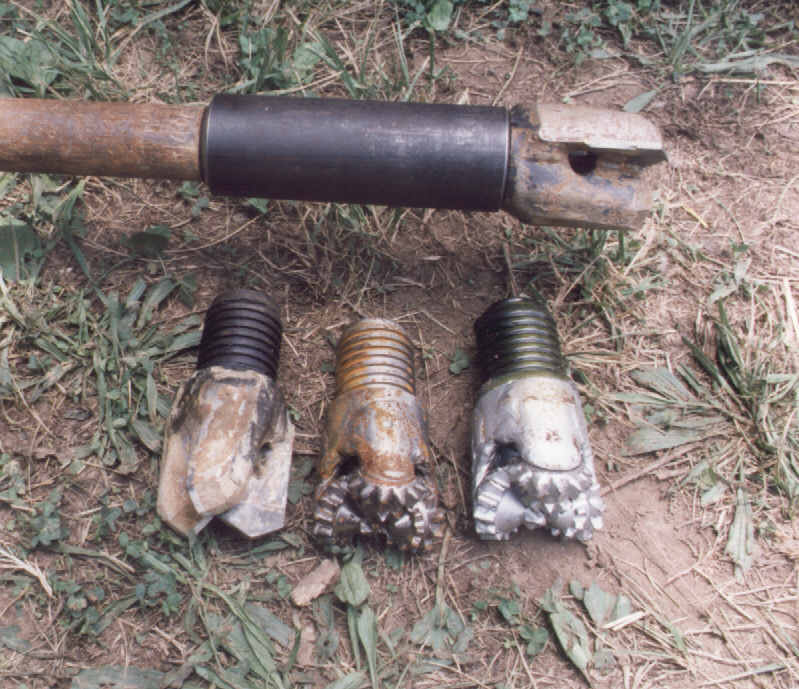
Figure 4a‐b: Drill bits used to make the pressuremeter test hole
- The driller should rotate the bit approximately 60 rpm. The engineer should draw a vertical mark on the rods and measure the rotation speed.
- The driller should circulate the drilling mud at a flow rate approximately 10 gallons per minute. To confirm the correct flow rate, the driller places a 5-gallon bucket under the flow discharge and uses a stop-watch to measure how long it takes to fill it. Figure 5 shows the driller using mud rotary to create the pressuremeter test hole.
- Depending on the soil conditions, the drill bit should advance continuously downward into the soil at a rate of 0.5 to 3 minutes per foot. The engineer should record the time for each foot of drilling, which may indicate the homogeneity or heterogeneity of the soil and guide the engineer to determine the best test depth.
- After finishing drilling the test zone, the driller may make one additional run up and down the hole to clean the hole, if the soil is not a loose sand.
- The driller should stop the mud flow and rotation, pull the bit up to the top of the run and then lower the bit to the bottom of the hole, ensuring the hole stays open to its bottom before lowering the pressuremeter probe.
- The driller should carefully lower the pressuremeter probe to the test depth and keep its cable taught, taping it to the sides of the rods at approximately 10 foot (3 meter) intervals.
- Fine tune the drilling technique based on the previous test results.
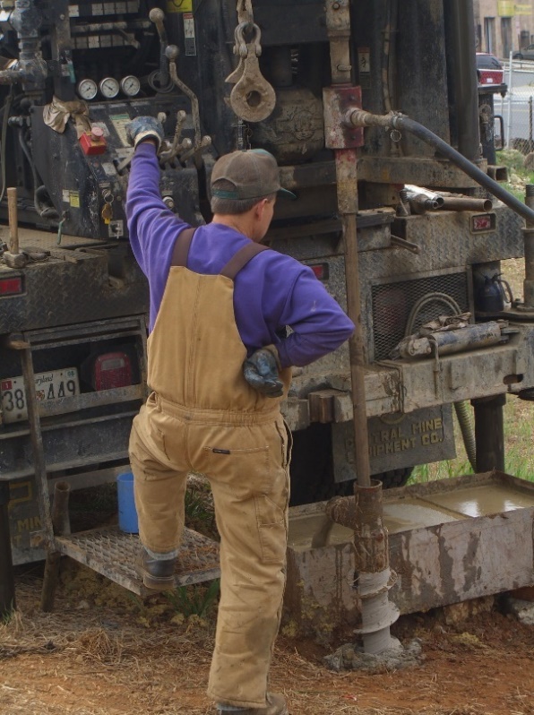
Figure 5: Ronald Stidham drilling a pressuremeter test hole
Performing a Strain-controlled Pressuremeter Test with the Texam Control Unit:
- The engineer should record the test depth below ground surface or the mudline and the height of the pressure gauge above the ground surface or mudline.
- He/she should inflate the pressuremeter probe in equal volume increments of 40 cm3 until the pressure becomes asymptotic with the volume increase or a maximum volume of 1600 cm3. After reaching a volume, the engineer, using a stopwatch, should wait 5 seconds and then record the pressure and volume. By waiting 5 seconds, the engineer ensures that the pressure at the gauge will be the same as in the probe, by eliminating the time lag.
- He/she finds the elastic portion of the PMT curve when the pressure increases in 3 or 4 equal increments for the equal volume increments of 40 cm3.
- After making the fourth measurement on the elastic portion, the engineer should perform an unload-reload loop using 10 cm3 increments, first by decreasing the volume 20 cm3 and then increasing back to the original volume. Figure 6 shows a typical high- quality pressuremeter test.
- After resetting the stop watch and injecting the next 40 cm3 volume increment, the engineer performs a creep test. He/she starts the stop watch and takes the pressure measurement after 5 seconds.
- He/she holds that pressure for 10 minutes and measures the pressuremeter volumes at elapsed times of 0.5, 1 ,2, 4, 7, and 10 minutes. To maintain that pressure, he/she will need to slowly and constantly inject volume over time. For a ten-minute long creep test the engineer should expect a volume increase of about 10 cm3 in cohesionless soil and up to 80 cm3 in cohesive soil.
- He/she inflates the pressuremeter to the next 40 cm3 volume increment, getting back to an even volume.
- The engineer should perform two additional unload-reload loops at 200 and 400 cm3 more than the first one.
- He/she continues to inflate the pressuremeter to a minimum of 1000 cm3 or maximum of 1600 cm3, until the pressure-volume curve has become nearly asymptotic with pressure.
- The engineer deflates probe back to zero volume, waiting for the pressure to decrease from about -0.9 bars (near vacuum) to about zero. Drilling fluid should fill the casing or hollow stem augers.
- Sometimes hard over-consolidated clays may adhere to the pressuremeter membrane preventing it from deflating, which the engineer observes if the membrane does not fully deflate after about 5 minutes. He/she should then increase the volume from zero to the volume that has zero pressure to determine the inflated size of the membrane. The driller should raise the pressuremeter probe about 1 inch (2.5 cm), squeezing the membrane. After waiting about 1 minute, the engineer should check the new size of the pressuremeter membrane at zero pressure. The driller and engineer should repeat this process until the membrane has fully deflated. By lifting the pressuremeter probe, the adhesion between the clay and the pressuremeter membrane will release
- After each test, the engineer should inspect and clean the membrane and remove all soil from between the metal protective strips to extend the life of the membrane.
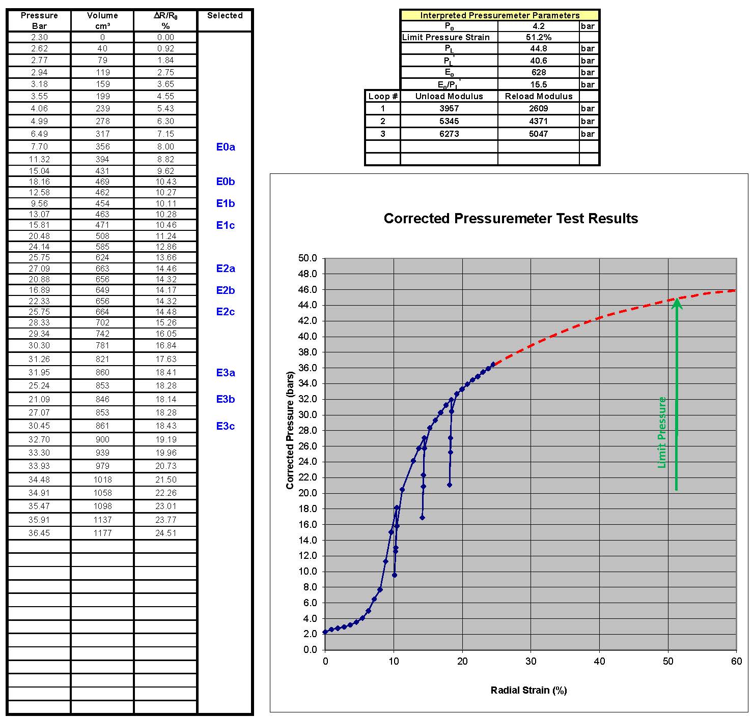
Figure 6: Typical pressuremeter test results
Calibration and System Checks:- Because water does not compress significantly under pressure, it makes the volume measurements. The engineer must confirm that the pressuremeter system has only water and no air in it. After disconnecting the pressuremeter probe and tubing from the control unit, he/she can exert about 25 bars of pressure and the resulting volume should approximate 14 to 18 cm3. If the volume exceeds 18 cm3, the system contains some air, which must be removed.
- The monocell membrane for the Texam pressuremeter has a bleed fitting at its bottom. By pointing the probe with its bottom up, the engineer can inject water through the tubing and probe until only water comes out of the bleed fitting. He/she should place his/her finger over the bleed port and inject an additional 300 cm3 of water, inflating the membrane. By tapping the sides of the membrane several times, any air bubbles that were clinging to the membrane will dislodge and travel towards the bleed port. The engineer then releases his/her finger and watches as initially some air bubbles come out followed by only water. He/she now knows that the pressuremeter system has only water in it and reconnects the bleed port cap fitting.
- The pressuremeter probe should have an initial volume so that it snuggly fits into its thick-walled steel calibration tube. For the Texam N-sized (73.8 mm) membrane inside its (76.2 mm) calibration tube, if pressurized to 5 bars, the pressuremeter will have a volume of about 180 cm3 for it to have a snug fit. The engineer may need to either add or remove water from the system to get to the initial volume.
- If the engineer places the pressuremeter probe inside the thick wall calibration tube and inflates the membrane to a pressure of 100 bars, he/she can confirm that the system has no leaks if little pressure deceases occur as the system creeps and shapes to the steel tube. Figure 7 shows the pressuremeter probe inside the thick-walled calibration tube.
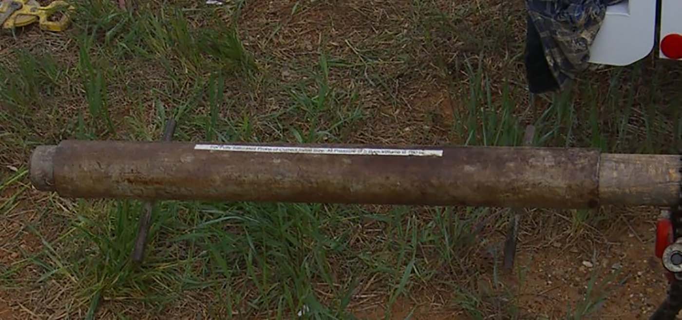
Figure 7: Pressuremeter probe inside thick‐walled steel calibration tube
- As pressures increase, the tubing will swell and the membrane will compress. During a test, the volume of the membrane that expands into the soil will equal the total measured volume less the volume that the tubing swells and membrane compresses. By placing the pressuremeter probe inside the thick-walled steel tube, the engineer should apply recommended pressures of 5, 10, 15, 20, 25, 30, 35, 40, 45, 50, unload to 25, reload to 50, 60, 70, 80, 90, and 100 bars and measure/record their corresponding volumes. The tubing swelling and membrane compression have a linear pressure/volume relationship. If the membrane has stainless steel protective strips adhered to its outside, for approximately the first 30 bars of pressure, the stainless-steel strips bend to fit the calibration tube and the linear pressure/volume relationship occurs after 30 bars. Because the tubing has different swelling and collapsing properties, the engineer uses a reload factor based from the unload reload calibration loop to correct the volumes for unload/reload cycles during a pressuremeter test. Longer lengths of tubing have higher volume calibration values. For a 100 foot (30 meter) long tubing, its calibration approximates 0.7 cm3/bar.
- Similar to blowing up a balloon, it takes more pressure initially to inflate it and less incremental pressure to inflate it more. The pressure that the soil feels during a pressuremeter test equals the measured pressure less the pressure needed to inflate the membrane in air. The engineer should inflate the pressuremeter membrane in air, at the approximate height as the pressure gauge, in 100 cm3 intervals and measure the corresponding pressures until the volume of the membrane has almost doubled (for the Texam N-sized membrane, this volume is 1600 cm3). The calibration should take about the same time as performing a test, and thus the engineer should calibrate by inflating 100 cm3 increments every 30 seconds and measuring those pressures. At a volume of 1600 cm3, the calibration pressure approximates 0.50 bars. Figure 8 shows the pressuremeter membrane calibration at a volume of 1600 cm3.
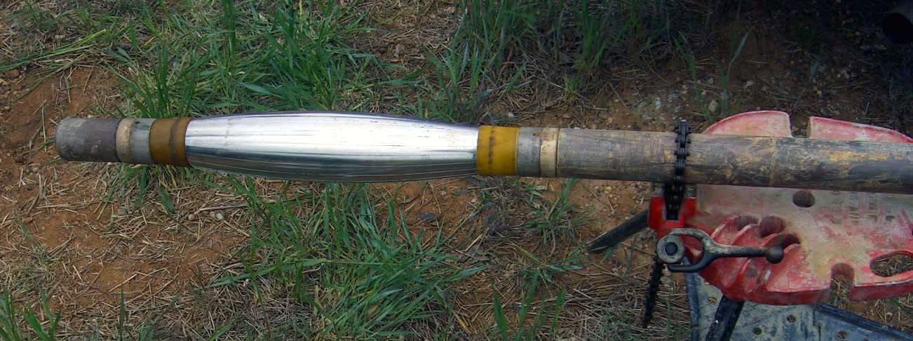
Figure 8: Membrane calibration at fully expanded volume of 1600 cm3
- The engineer should calibrate the pressuremeter probe every time he/she replaces the membrane. The calibration values do not change much with different membranes, but the length of the tubing affects the system calibration (the longer the tubing, the higher the calibration values). After several tests, however, sand grains can get lodged between the stainless-steel protective strips, making the probe too large to fit inside the thick-walled steel calibration tube and thus preventing the engineer from performing an additional system calibration.
Processing the Pressuremeter Test Data:
When performing the pressuremeter test, the engineer should find the elastic portion of the test by measuring equal pressure increments for 3 or 4 corresponding equal volume increments (40 cm3). He/she equates the final data point on the elastic portion and start of the plastic portion of the pressuremeter curve as the pressuremeter yield point, γ. After reaching the yield point, he/she should perform an unload-reload cycle by decreasing the volume in 10 cm3 increments twice and then reloading in 10 cm3 increments twice [-10, -20, +10, and +20 cm3] back to the starting volume of the loop. During the test, the engineer should perform two additional unload-reload loops at initial volumes of 200 and 400 cm3 more than the first loop, so that he/she can measure the soil’s stain hardening properties.
At the next volume increment after the first unload-reload loop, the engineer should perform a creep test by maintaining the pressure for ten minutes. He/she resets the stopwatch and starts it after injecting the fluid volume. The engineer records the pressure 5 seconds after reaching the volume to avoid time lag error and then holds that pressure constant by injecting more volume and records the volume at 0.5, 1, 2 ,4 ,7, 10 minutes. He/she plots log10(measured volume – initial volume of the pressuremeter contacting the sidewalls of the borehole) as the y-axis versus log10(elapsed time) as the x-axis (Figure 9). Using linear regression, the engineer determines the slope of the best fit line as the “n” coefficient and computes its coefficient of determination, r2, which almost always exceeds 0.98. For cohesionless soil, n ranges from 0.005 to 0.03, while for cohesive soil, n ranges from 0.03 to 0.08. Because the engineer measures the pressuremeter modulus in about one minute, he/she can compute the modulus for the design life of the structure using the following formula:
E0(design life time in minutes) = E0(time=1 min) * (design life time in minutes/1 minute)-n
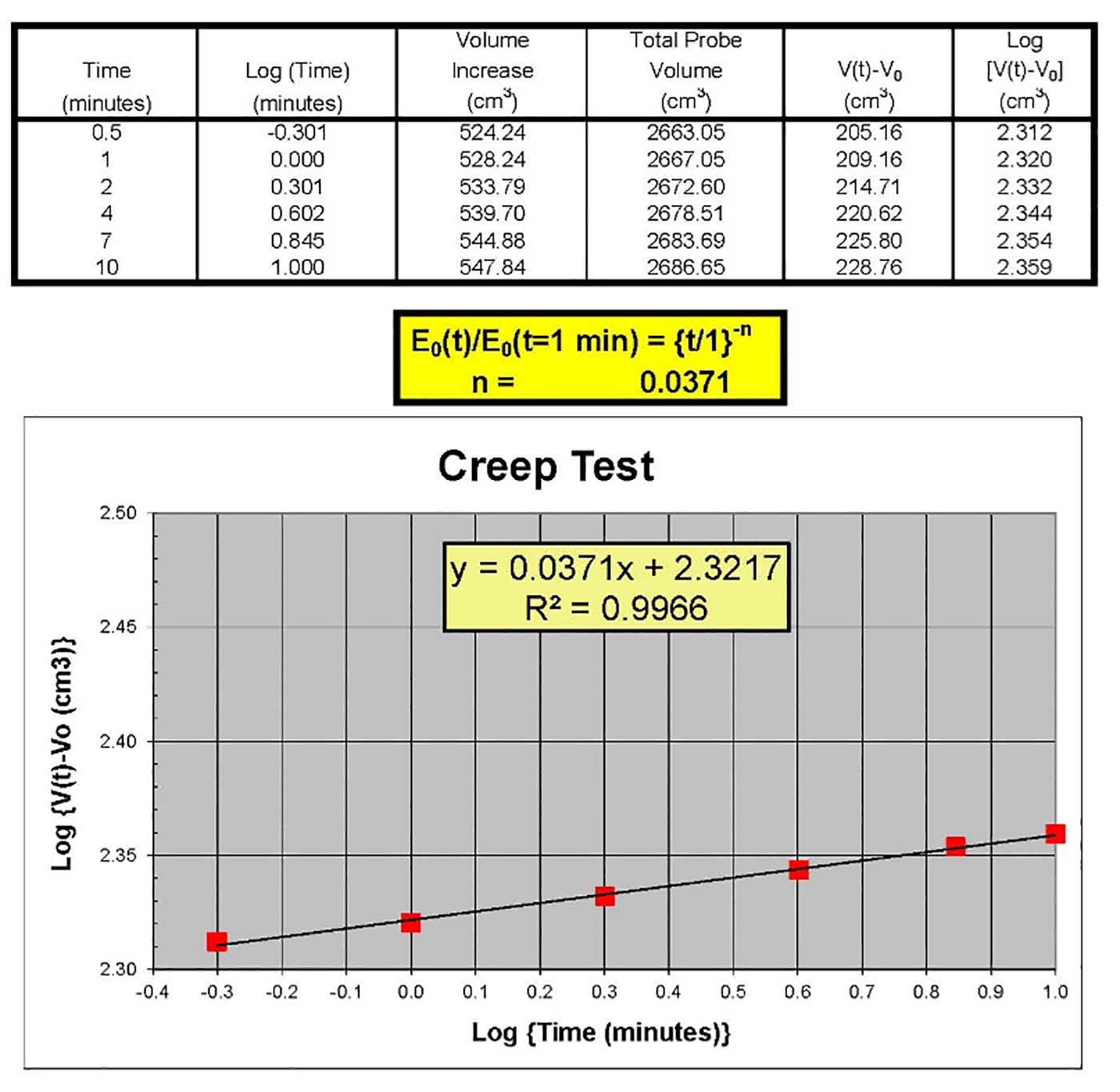
Figure 9: Typical creep test results
The engineer can perform pressuremeter tests in sand, gravel and occasional cobble formations using a slotted casing pressuremeter (Figure 10). In this case, he/she places an “A” sized probe (1.73 inch/44 mm diameter) inside a section of BX casing (2.5 inch/63.5 mm) that has 12 laser-cut longitudinal slots through the casing (30 degrees apart) allowing the steel casing to expand. Using the procedures described above, the driller mud rotary drills with a 2.5 inch (63.5 mm) diameter bi-cone bit to create the test zone. Due to the large sized gravel and occasional cobbles, the borehole may become somewhat crooked and the driller cannot simply lower the slotted casing pressuremeter but must lightly tap it into the test zone with his/her SPT hammer. If the driller must impact the slotted casing pressuremeter with heavy blows, then the test zone likely has protruding cobbles/boulders and the test will likely not have success. The engineer must stop inflating the slotted casing pressuremeter at a maximum volume of 800 cm3, otherwise he/she will cause permanent deformation to the slotted casing. Additionally, he/she should use volume increments of 20 cm3 instead of 40 cm3 for the test. Because of the large sized soil particles, not every test will succeed and any zones with boulders will result in an unsuccessful test. Farouz and Failmezger (2006) showed the slotted casing pressuremeter tests in these large-sized, difficult to test soils can result in large cost savings for foundation design that relies on knowing their strengths and stiffnesses.
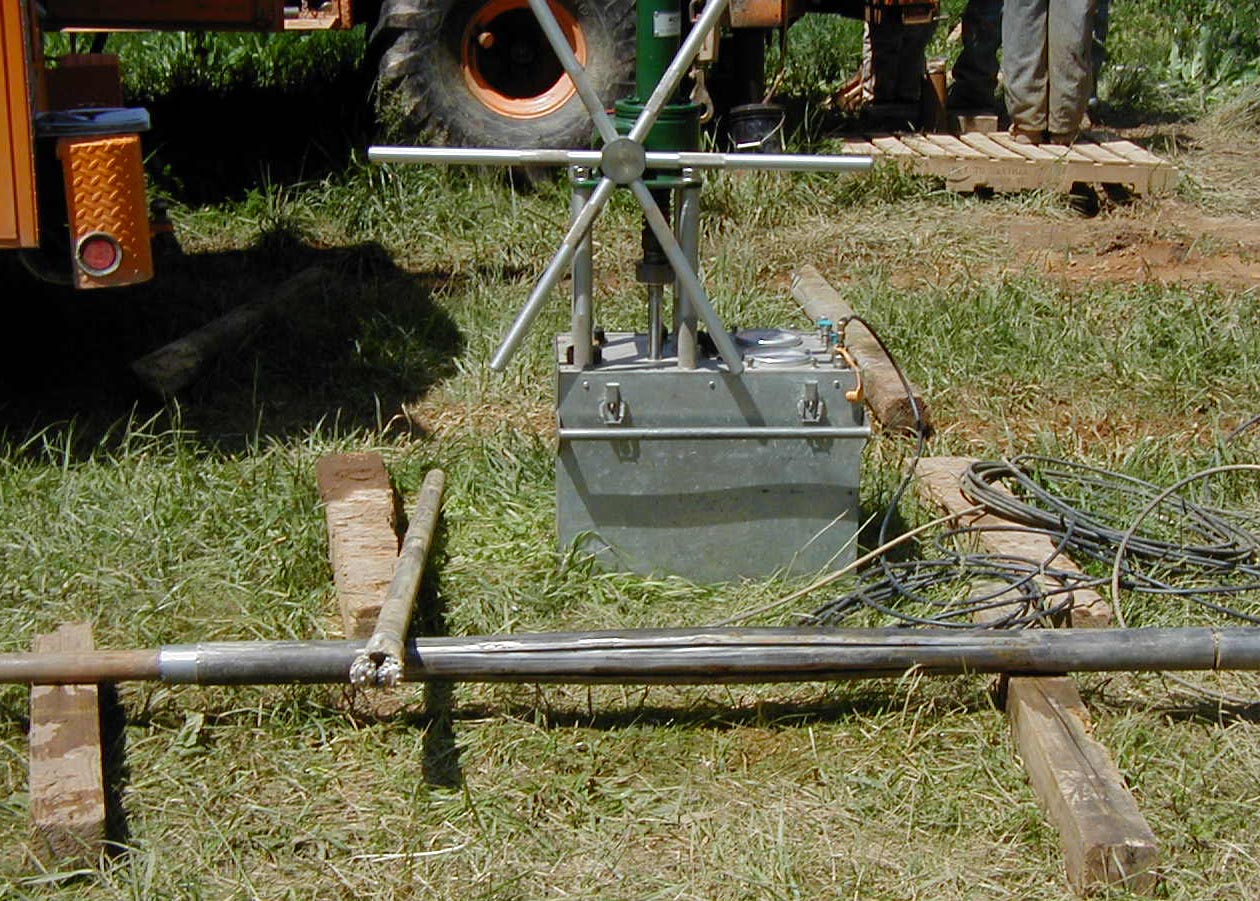
Figure 10: Slotted casing pressuremeter expanded to 800 cm3 and bi-cone drill bit
The engineer can use an Excel file to process the field pressuremeter test data.
Interpretation of Pressuremeter Test Results
After correcting for pressure and volume losses using their membrane resistance in air and probe in thick-walled steel pipe system calibrations, the engineer plots the corrected pressure test results as applied pressure versus radial strain. The resulting plot shows up to five distinctive portions which characterize the stress-strain behavior of the soil, namely:
- The borehole contact pressure or horizontal pressure at rest, ρ0H,
- The linear pseudo-elastic stress-strain portion of the deformation curve, defining the initial pressuremeter deformation modulus, E0;
- The departure from linear elastic conditions to plastic deformation starting at the yield pressure, ργ;
- The unload-reload portions of the test (usually three cycles are performed); and
- The development of soil failure, which is represented by limit pressure, ρL, which equals the pressure when the pressuremeter has doubled in size from its contact with the borehole sidewalls. The net limit pressure ρ*L, which equals the limit pressure minus horizontal pressure at rest.
Based on these test features the engineer determines or estimates the following soil parameters:
Contact Pressure ρ0H:
- When using the prebored TEXAM unit, the engineer computes the initial contact pressure as the pressure at the intersection of the two lines representing the pseudo elastic (red) and the initial expansion (green) portions of the pressure versus radial strain, as shown on Figure 11. Furthermore, that point represents the radial strain at contact.
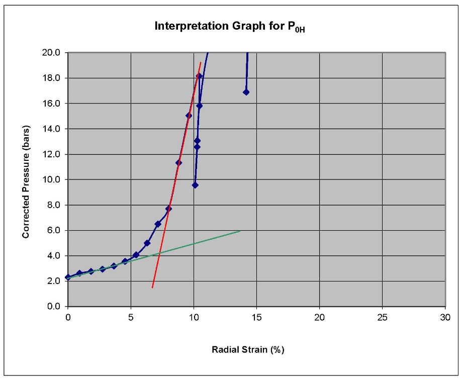
Figure 11: Interpretating Ρ0H
Pressuremeter modulus EPMT or Eo:
The engineer computes the pressuremeter modulus by multiplying the slope of the pressure versus radial strain curve along its linear portion by (1 + poisson’s ratio), as follows:
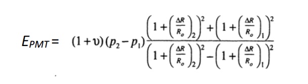
Εwhere the sub-indices 1 and 2 indicate the beginning and the end of the linear portion of the curve, respectively. For a self-boring pressuremeter test, the linear portion of the stress-strain response occurs between the first data point (zero volume increase) and the subsequent two or three data points. The engineer assumes a value of the Poisson’s ratio, typically ν = 0.33 for most soils for the above formula.
Because the Pressuremeter modulus ΕPMT corresponds to large strains, namely for radial strains in the 2 to 5 % range, it represents a relatively low value of the elastic modulus. In practice, the Young’s modulus E can be inferred from Pressuremeter testing using the Menard α factor:
Ε = ΕΡΜΤ/α
The engineer can choose the Menard α factor from Table 1 or Figure 12:
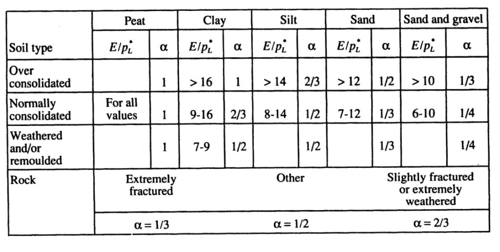
Table 1: Typical Menard α factors (from ‘The Pressuremeter’, J.L. Briaud. Balkema, 1992)
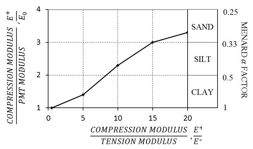
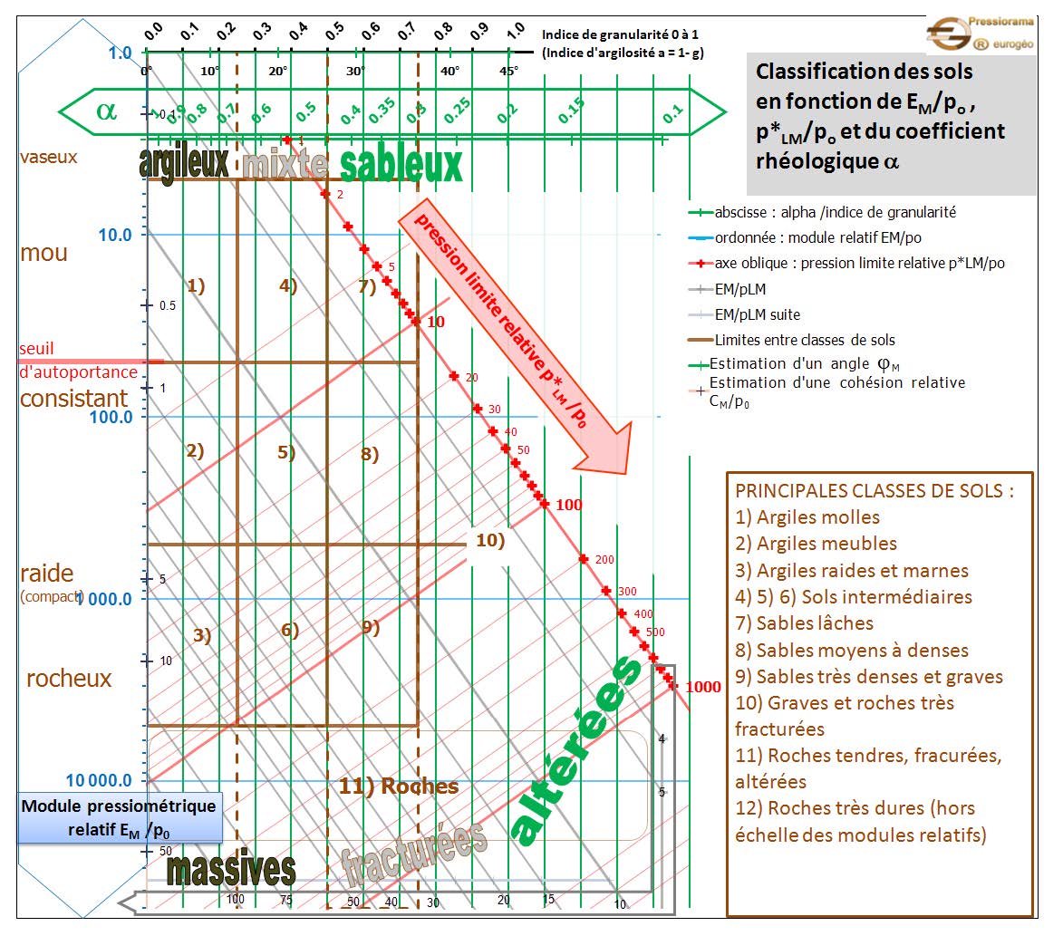
Figure 13a [Français]: Proposed Menard α factors from Baud J.P., and Gambin M. 2013. “Détermination du coefficient rhéologique α de Ménard dans le diagramme Pressiorama”. Proceedings of the 18th International Conference on Soil Mechanics and Geotechnical Engineering. Paris, 2013, Parallel Session ISP 6, International Symposium on the Pressuremeter
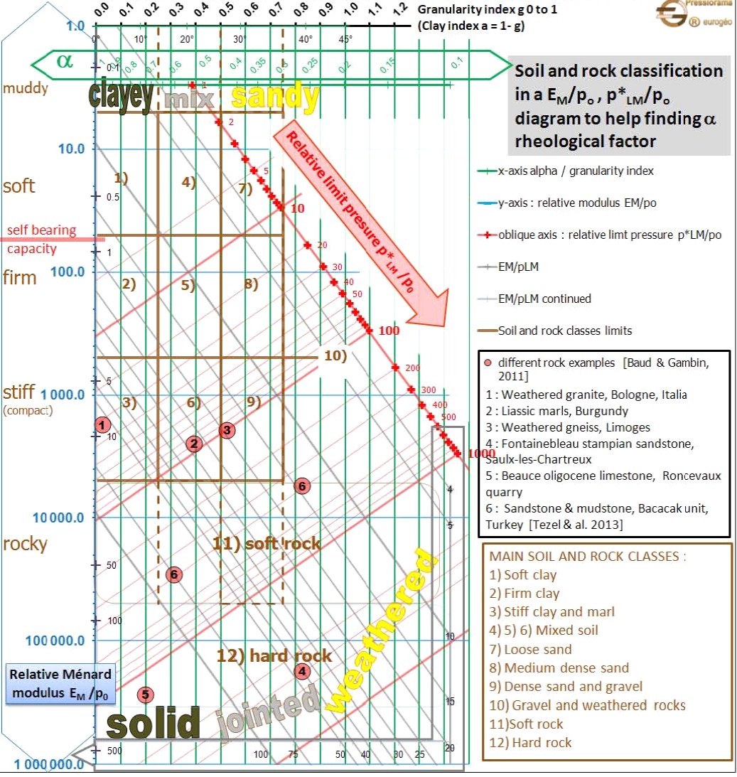
Figure 13b [English]: Proposed Menard α factors from Baud J.P., and Gambin M. 2013. “Détermination du coefficient rhéologique α de Ménard dans le diagramme Pressiorama”. Proceedings of the 18th International Conference on Soil Mechanics and Geotechnical Engineering. Paris, 2013, Parallel Session ISP 6, International Symposium on the Pressuremeter.
- Yield Pressure ργ:
The yield pressure signifies the end of the linear pseudo-elastic deformations and the onset of plasticity. The engineer uses the yield pressure to indicate that pressures exceeding it may have significant creep deformations. Design bearing pressures for shallow foundations should not exceed the yield pressure.
- Unload-Reload Moduli ER and EU:
The engineer calculates the reload and unload moduli by multiplying their respective slopes of the unload-reload loop by (1 + Poisson’s ratio). He/she uses these values to determine elastic soil deformations upon unloading conditions such as those typically encountered during excavations. With multiple unload/reload loops, the engineer may model strain hardening of the soil.
- Limit Pressure pL /Net Limit Pressure p*L:
The limit pressure, PL, equals the pressure when the soil cavity has expanded to twice its original volume. The net limit pressure, PL*, equals the limit pressure minus the initial contact pressure poH. The net limit pressure measures the strength of the soil (either under undrained conditions for cohesive soil, or drained conditions for cohesionless soil). The engineer can compute the radial strain for the limit pressure using the following equation:
Radial Strain at PL = 0.41 +1.41 * Radial Strain at P0H
The engineer should continue to inflate the pressuremeter until he/she has clearly failed the soil and the pressure becomes asymptotic to the limit pressure with increased radial strain. He/she can extrapolate the corrected pressuremeter test to the calculated radial strain for the limit pressure either by eyeballing the curve or using a second, third or fourth order polynomial curve fit. We prefer the eyeballing method as it seems to include engineering judgment.
As a second method, the engineer can plot pressure versus 1/V for the plastic phase of the deformations and extrapolate out to the limit pressure. This second method, also named the “upside down curve” method, is described in “The Pressuremeter and Foundation Engineering” textbook, by F. Baguelin, J. F. Jezequel, and D. H. Shields, published in 1978 by Trans Tech Publications, Section: Methods of extrapolating pressuremeter curves to ρL.. See also ASTM D4719-00, Section 10.6.
- Creep Factor, n
By holding the pressure constant by adding volume over time (typically 10 minutes), the engineer computes the creep factor, n, as the slope of the line from the plot of log10(net volume more than the initial volume) [y-axis] versus log10(elapsed time) [x-axis]. When performing settlement analyses, the engineer should either reduce the modulus or increase the total predicted settlement using the below formulas:
E0(design life time in minutes) = E0(time=1 min) * (design life time in minutes/1 minute)-n
Settlement(design life time in minutes)= Settlement(time = 1 minute) * (design life time in minutes/1 minute)n
- Some Additional Parameters
for sands
7 < EPMT / ρ*L < 12
0.005 < n < 0.03
for clays
12 < EPMT / ρ*L
0.03 < n < 0.08
Also, the Canadian Foundation Engineering Manual (4th Edition, 2006) suggests the following ranges for pressuremeter parameters (Table 2).
For most soil types the ratio between the limit and the yield pressures may be expressed as:
1.3 < (ρ*L / ρy) < 2.0
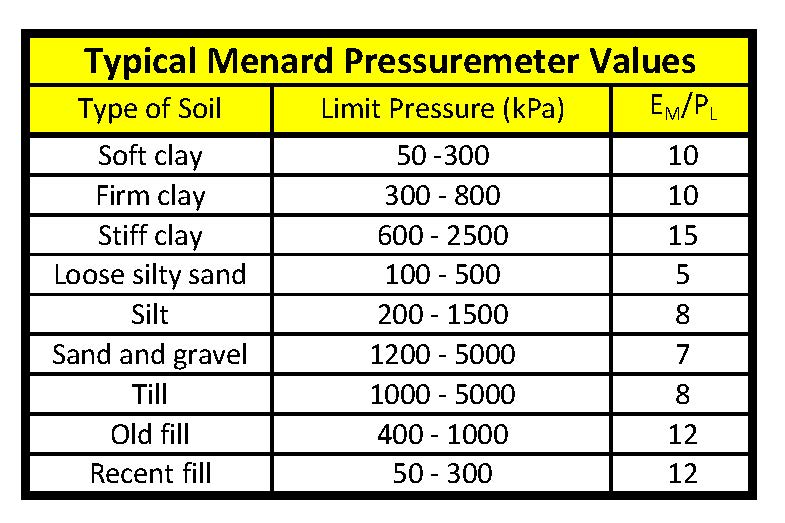
Table 2: Typical Menard Pressuremeter Values (Canada)
Also as a general guideline, Briaud suggests clays and sands may have the following parameters: (Table 3)
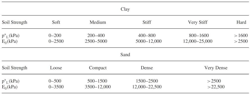
Table 3: Typical Net Limit Pressures and Moduli Value for Clays and Sands
Judging the Quality of the Pressuremeter Test:
Figure 14 (Briaud 1988 FHWA Manual) shows example of good quality pressuremeter tests for sands and clays. Clays clearly fail with increased radial strain, while sands fail more gradually.
Figure 14: Examples of high quality pressuremeter tests for clay and sand
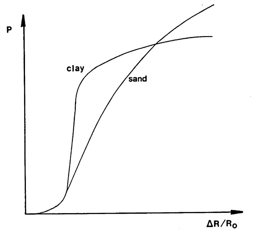
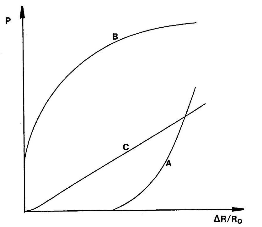
Figure 15 (Briaud 1988 FHWA Manual) shows example of poor quality pressuremeter tests caused by poor borehole preparation. For Case “A” the borehole is too large and the modulus may be interpreted but the limit pressure cannot be interpreted. For Case “B” the borehole is too small and the modulus may not be interpreted due to soil disturbance but the limit pressure may be interpreted. For Case “C” the soil has been disturbed during drilling and neither the modulus or limit pressure can be interpreted. The engineer and driller should make adjustment to the drilling procedure so that high quality test holes, like those in Figure 14, are made eliminating interpretation uncertainty from poor quality boreholes.
Figure 15: Poor quality tests from poorly made boreholes
Shear Strength Parameters
The engineer may predict the undrained shear strength of cohesive soils from the following equation:
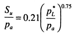
where ρα represents a reference pressure (i.e., atmospheric pressure = 100 kPa), after J.L. Briaud (‘The Pressuremeter’, Balkema, 1992).
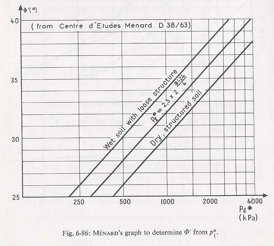
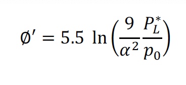
The drained friction angle of cohesionless soils (c’ = 0) may be estimated using the empirical correlations illustrated in the graph shown on Figure 16. This approach is outlined by Baguelin et.al., in “The Pressuremeter and Foundation Engineering” (F. Baguelin; J.F. Jézéquel; and D.H. Shields. TransTech Publications. 1978), and it requires some knowledge on the state or conditions of the cohesionless material. This approach only provides a likely range of friction angles from interpreted limit pressure values.
Figure 16: Estimating angle of internal friction from net limit pressure
![Modified Pressiorama Chart to compute angle of internal friction [Français]](https://insitusoil.com/wp-content/uploads/2022/02/Soil-pressuremeter-test-figure-17a-modified-pressiorama.png)
Figure 17a: Modified Pressiorama Chart to compute angle of internal friction [Français]
![Modified Pressiorama Chart to compute angle of internal friction [English]](https://insitusoil.com/wp-content/uploads/2022/02/Soil-pressuremeter-test-figure-17b-modified-pressiorama.jpg)
Figure 17b: Modified Pressiorama Chart to compute angle of internal friction [English]
Conservative estimates (lower‐bound estimates) of strength parameters can also be inferred from Table 4:
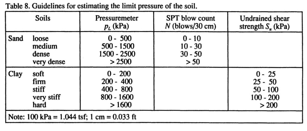
(from ‘The Pressuremeter’, J.L. Briaud. Balkema, 1992)
Table 4: Estimates for limit pressures
Design of Shallow Foundations:
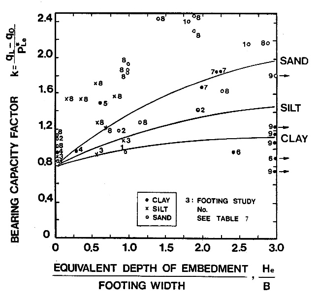
With pressuremeter data, the engineer can design shallow foundations using bearing capacity and settlement criteria. For bearing capacity criteria, he/she designs based on an equivalent net limit pressure within 1.5 times the footing width above and below the footing depth and uses the following equation for the ultimate bearing capacity.
qL = (k)(ρLe*) + q0
where k can be obtained from Figure 18—Briaud (2021) suggests using k =0.9 for clay or k = 1.2 for sand
pLe* = equivalent net limit pressure, and
q0 = total stress overburden pressure at the footing depth.
The engineer can compute settlement using either 1) the Menard and Rousseau (1962) method or 2) Briaud (2013) method. For the Menard and Rousseau method, he/she uses the following equation where the first term represents deviatoric settlement and the second term represents spherical settlement.
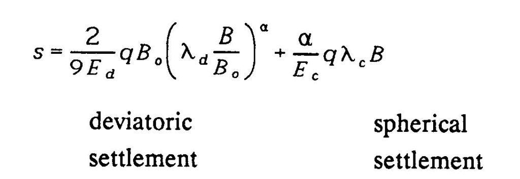
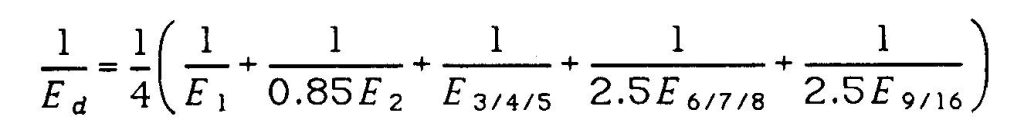
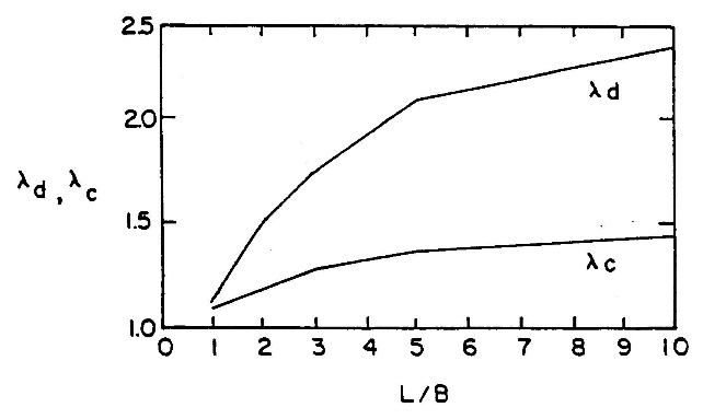
Figure 19: Menard’s shape factors
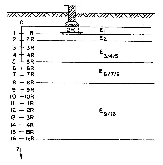
Because the modulus is a denominator term in the settlement computation, he/she must use a geometric mean rather than the mean or average value.
Figure 20: Calculation of Ed
The Briaud method uses the entire pressuremeter test curve to simulate a footing load test with calculations shown on Load Settlement Curve Method Excel spreadsheet. Instead of using empirical α factors to evaluate time dependent settlement, the engineer uses the measured creep factor, n. Figure 21 shows how well Briaud’s method compares with load test results from different width footings.
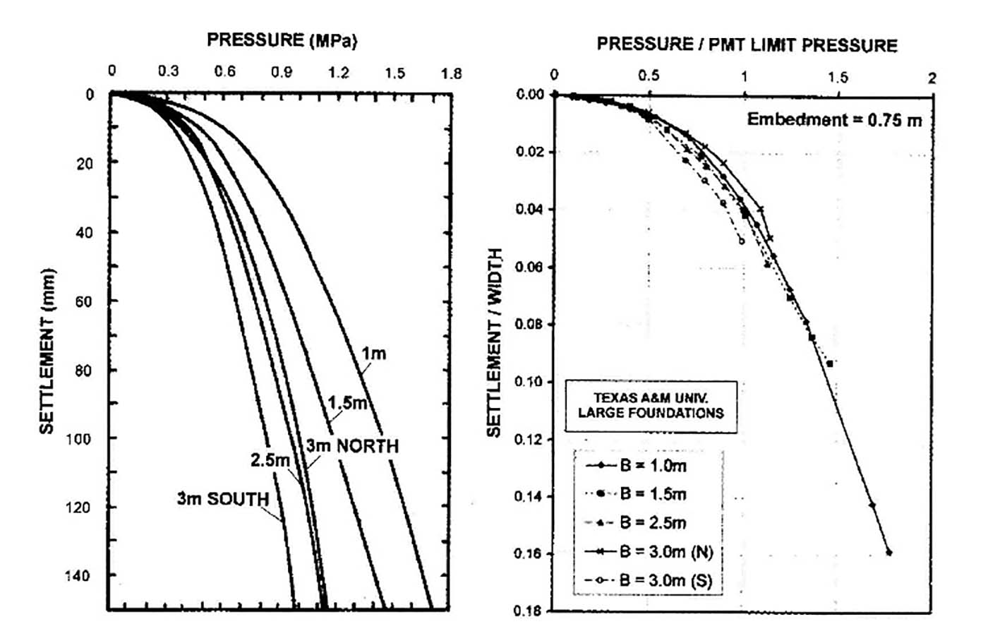
Figure 21: Briaud method‐‐comparison with footing load tests
Design of Deep Foundations
The engineer designs the vertical capacity of a deep foundation based on the pressuremeter limit pressure. He/she computes the frictional capacity using the following equation and obtains the correlation factors from Table 5 and Figure 22 depending on the soil type:
fu = α * fsoil *As
where α = pile type/installation method factor
fsoil = frictional capacity of the soil/rock not exceeding recommended maximum value,
As = side or circumferential area of the deep foundation, and
fu = ultimate side shear resistance of the deep foundation.
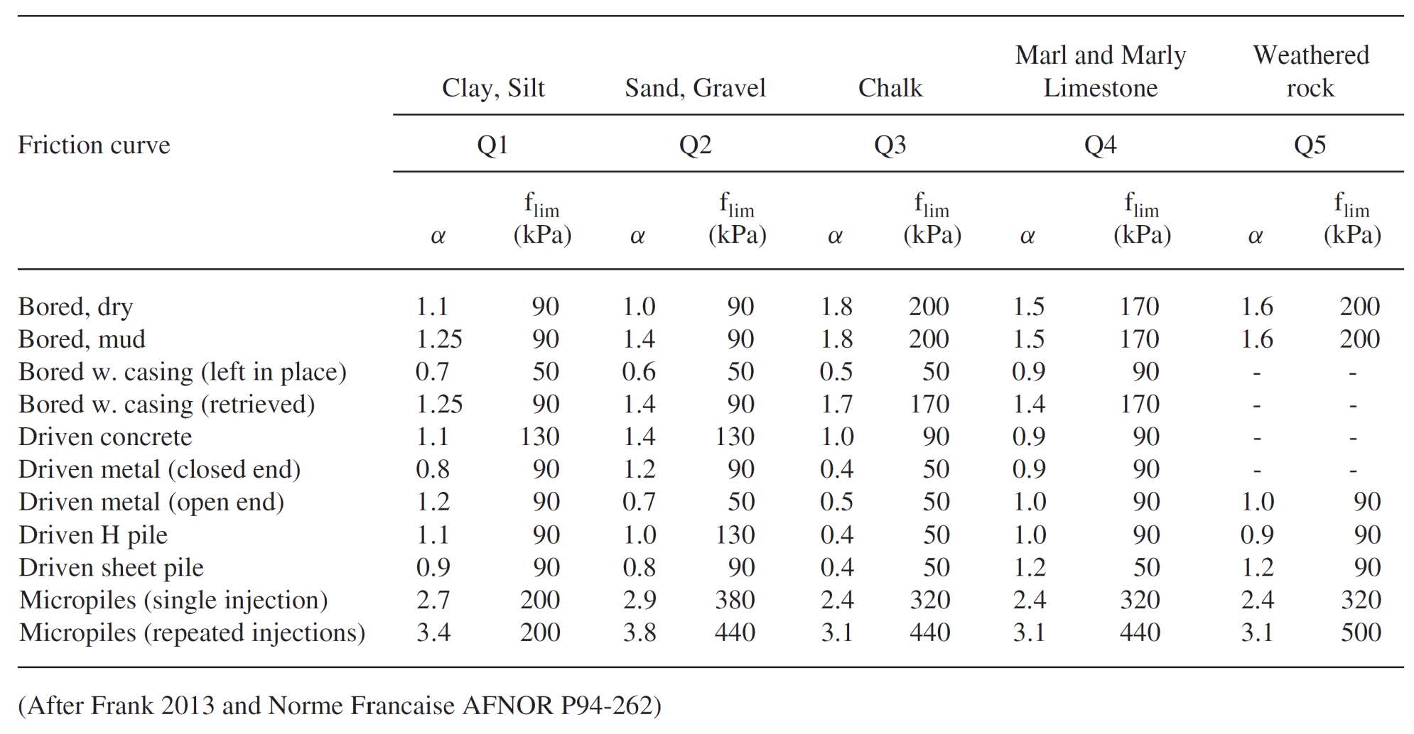
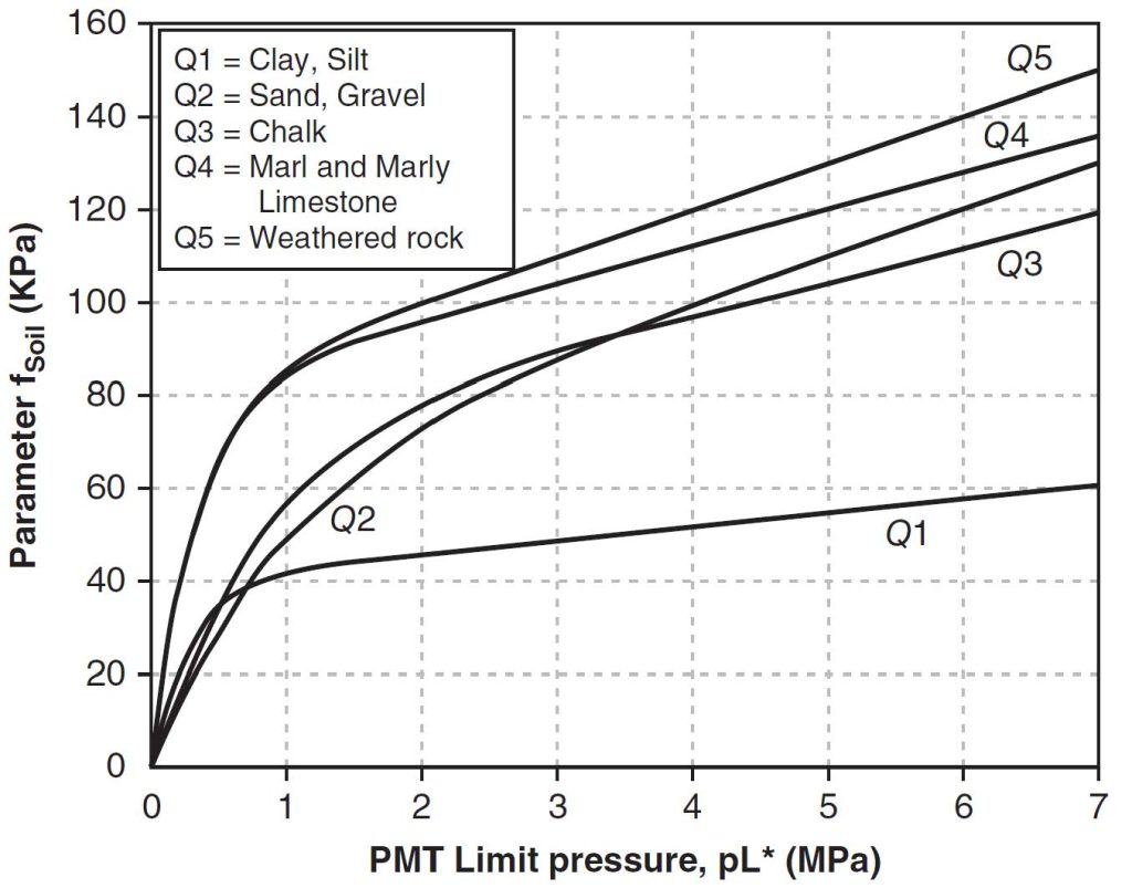
Figure 22: Soil friction resistances based on limit pressure and soil/rock type
The engineer computes the ultimate tip resistance using the following equation:
pu = [kp * pL + γ * d] * Ap
Where kp equals a bearing capacity factor (Table 5),
pL = the average limit pressure 1.5 * pile width/diameter above and below the tip,
γ = average unit weight,
d = pile tip depth,
Ap = tip area, and
pu = ultimate tip capacity.
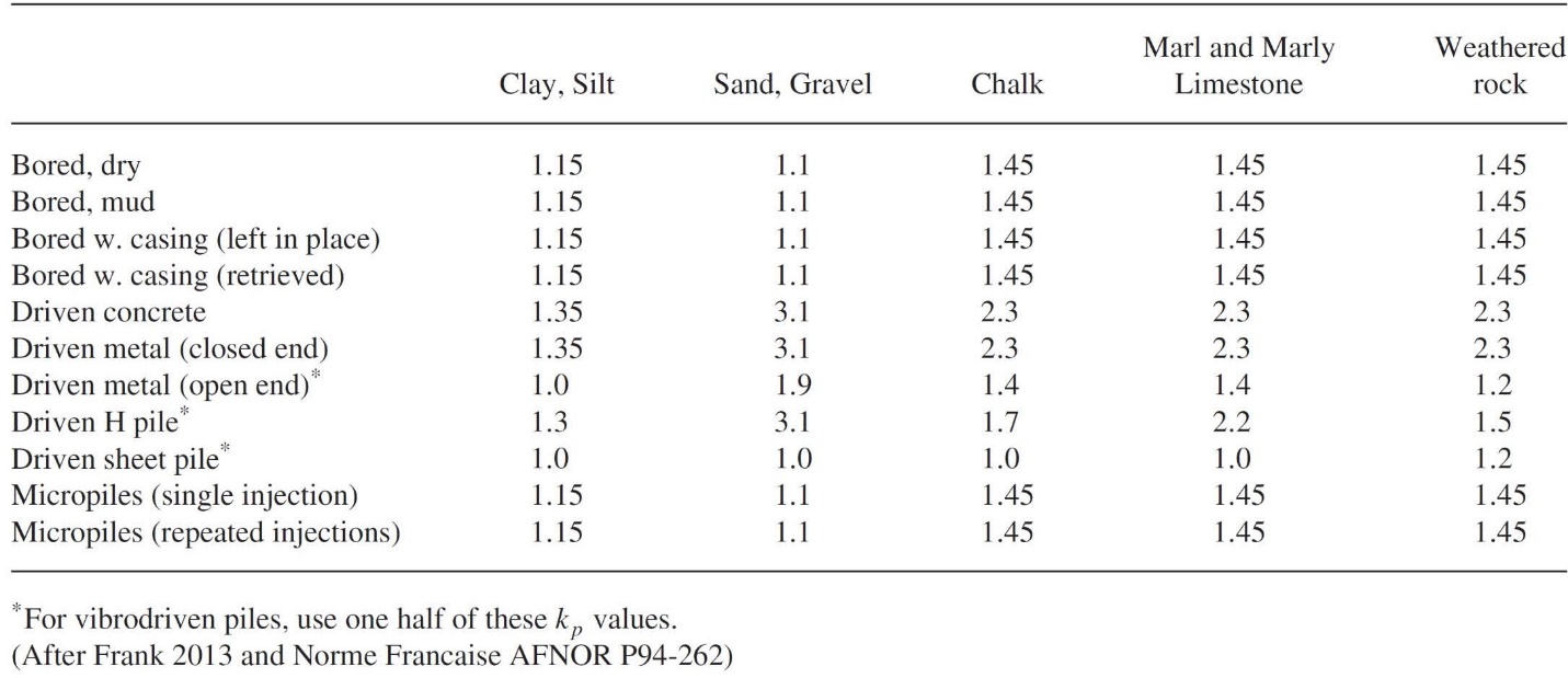
Table 6: Bearing capacity factors, kp, for deep foundation design
Lateral Load Capacity for Deep Foundations:
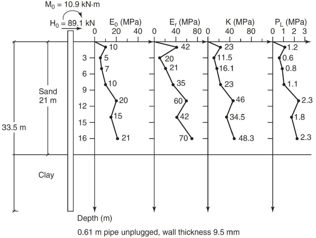
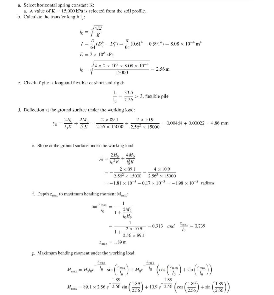
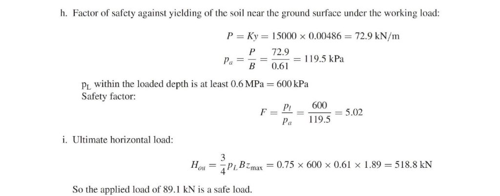
The pressuremeter laterally expands into the soil or rock and ideally models the lateral load capacity of a deep foundation. Briaud (2021) clearly explains the lateral load capacity analyses in Figures 23-28 and presents an example computation of a long flexible pile subjected to lateral loads.
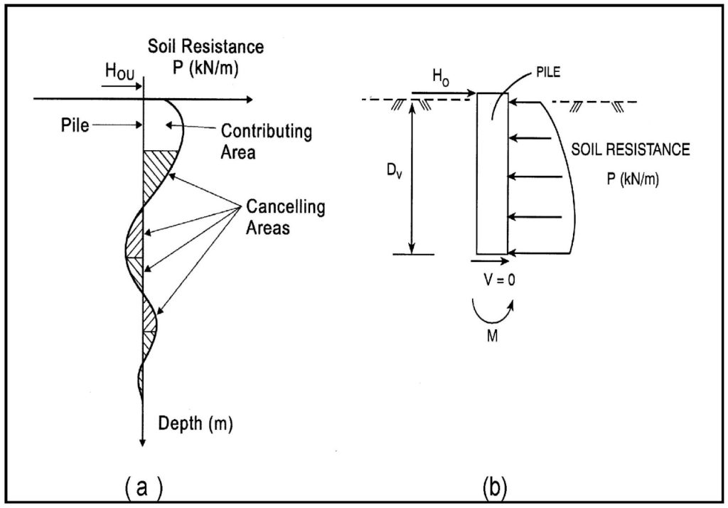
Figure 23: Lateral load resistance concept
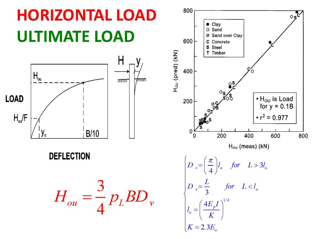
Figure 24: Computation of ultimate lateral capacity at deflection of B/10
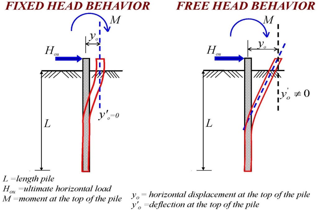
Figure 25: Fixed head versus free head behaviors
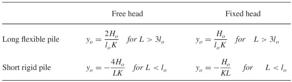
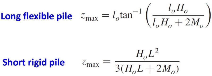
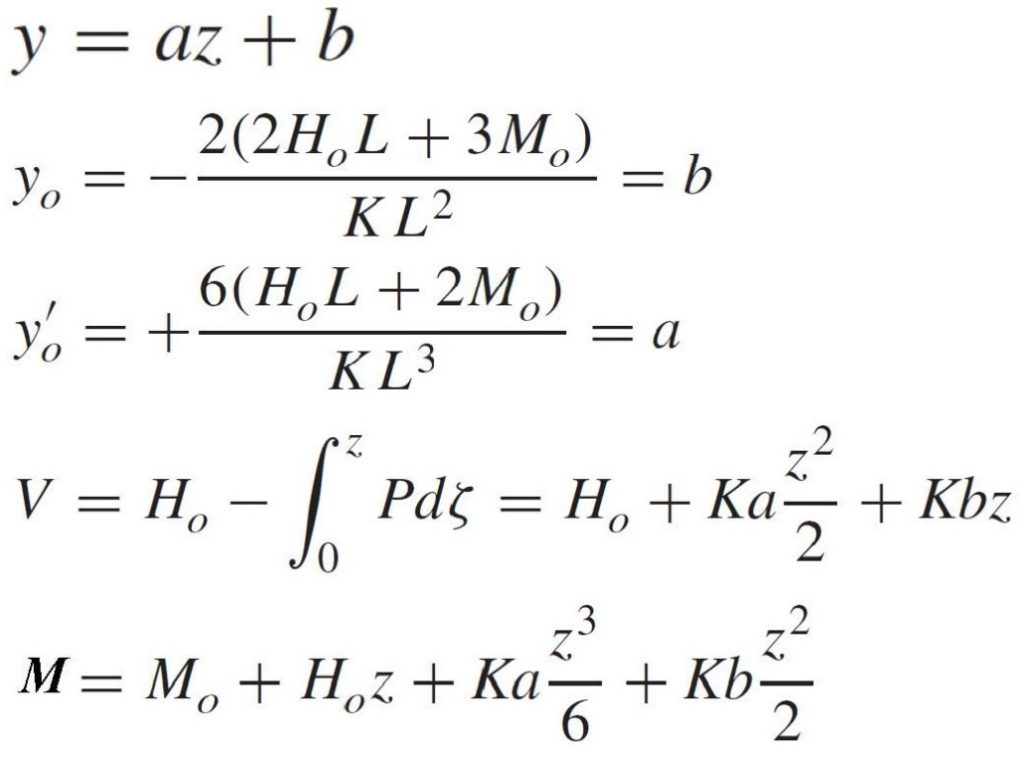
Figure 28: Lateral load formulas for deflection, slope, shear and moment