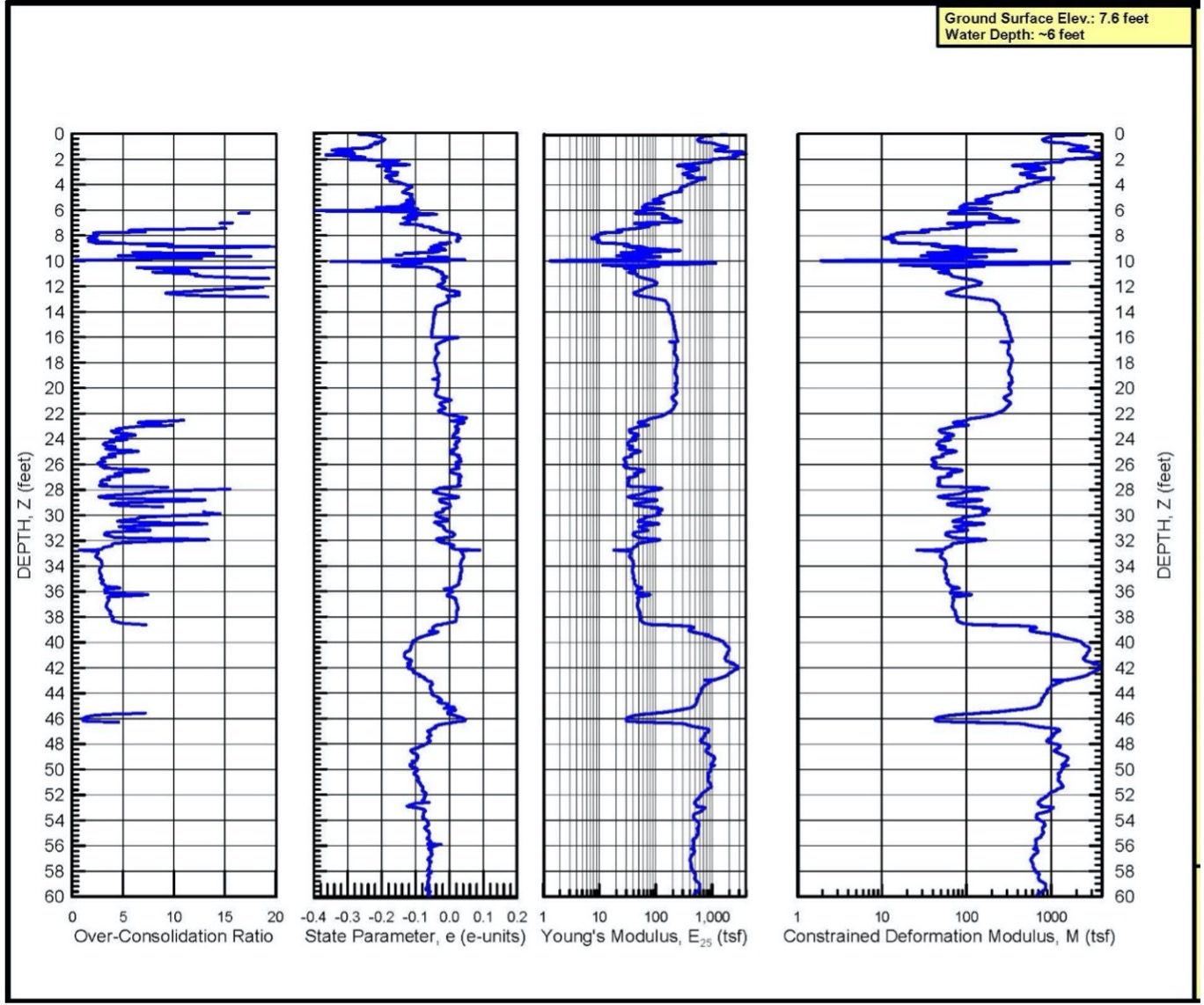
- Accurately profiles the geological strata
- Accurately predicts vertical pile capacity for deep foundations
- Measures the low strain shear wave velocity for seismic evaluations satisfying International Building Code (IBC) requirements
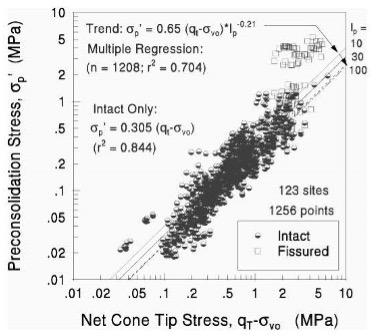
- Makes fair predictions of time rate of consolidation and permeability tests through pore pressure dissipation tests—good for wick drain design
- In normally consolidated or recently aged cohesionless soils, provides fair estimates of settlement for shallow foundations
In-Situ Soil Testing often performs CPT with the direct push truck that Dr. Schmertmann used for his pioneering research (Good Karma) [First direct push truck in North America—history]. To assure high quality control, a registered professional engineer performs the tests.
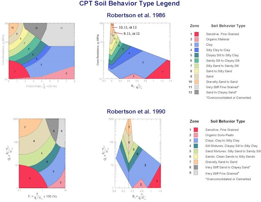
History of Cone Penetrometer Test (CPT), ASTM D 3441 and D 5778: The mechanical cone penetrometer probe, invented in The Netherlands in 1932 by P. Barentsen, measures the quasi-static thrust required to push a solid, conical tip having a 60 degree apex angle and a cross‑sectional area of 10 cm2 into the foundation soil. The operator advances the cone using a nested, dual‑rod system, the outer rods providing strength to penetrate the cone in a collapsed configuration, and the inner rods allowing him or her to advance only the cone tip at each test depth (generally at 20-cm intervals) while measuring the hydraulic thrust pressure at the top of the rods. In 1953, Begemann modified the probe to include a friction sleeve just behind the tip. For the friction cone test, the inner rods initially advance only the tip for a short distance, and then engage both the tip and a friction sleeve together. The unit soil adhesion acting on the center of the friction sleeve, located 20 cm above the tip, equals total thrust of the tip and friction sleeve minus the tip-only thrust force (from the previous test depth) and then divided by the sleeve area of 150 cm2. The engineer then divides the unit adhesion by the unit tip bearing from the previous test depth to determine the friction ratio (both readings then apply to the same depth). However, the term “friction” is a misnomer as it has no meaning to the shear strength of soil. Cohesionless soils that have higher shear strengths than cohesive soils have lower “friction ratios” than cohesive soils. Empirical charts identify the type of soil based on how it behaves either drained or undrained.
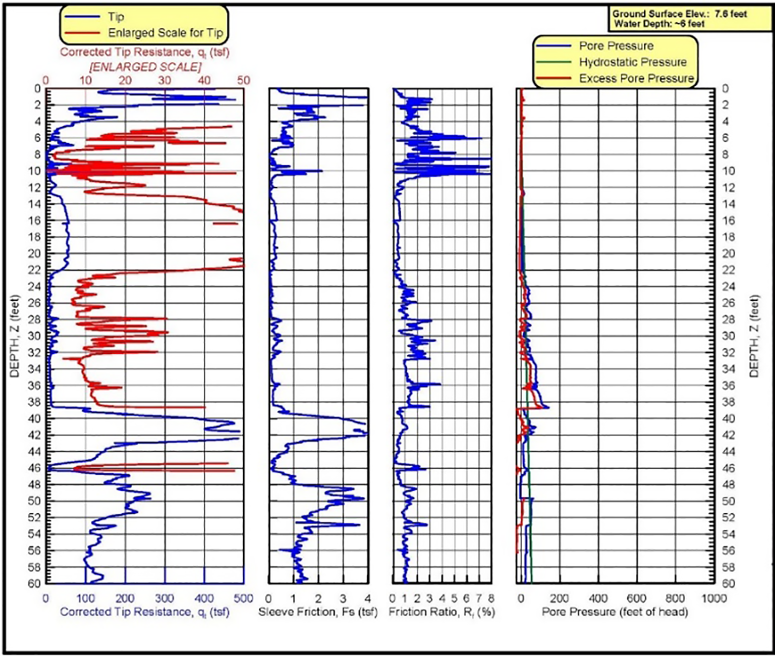
The improvement of electronics and computers in the 1980s led to the development of stainless-steel electrical cone penetrometer probes that obtain and record more reliable test measurements and eliminate the dual-rod system. Because the electric cones make measurements continuously instead of stopping every 20 cm as mechanical cones do, the electric cone soundings take slightly less time to perform than mechanical cone soundings. Strain gauges measure the tip and friction resistances and a pressure transducer measures the pore water pressures generated during penetration. With the electric cone, data are collected at penetration increments of 0.5 cm to 5 cm depending on the computer acquisition system (ours uses 1 cm) [Figure 1].
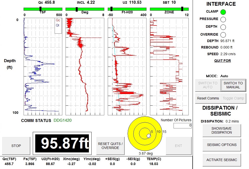
Figure 1: Screenshot of CPT data acquisition
Engineers prefer the electronic cone’s accuracy and productivity, relegating the mechanical cone to profiles containing strong materials that might damage the more expensive electrical cone. The cone penetrometer can penetrate soil with an N60-value of about 50 blows per foot with a 15 ton (13,000 kgf) direct push rig or soil with an N60-value of about 30 blows per foot with a 5 ton (4,000 kgf) heavy drill rig. The adapter that connects the cone to the push rods has a larger diameter than the push rods making a larger diameter hole and minimizing soil adhesion along the push rods (named a friction reducer).
By monitoring the inclination sensors, the engineer can follow the data collection computer screen’s graph of inclination versus depth as the CPT probe advances into the soil. Anomalies, such as cobbles, concrete or bricks, can cause the probe to deflect significantly. After disconnecting the depth recording cable, the engineer can cycle the probe up and down the sounding. Often, the probe will resume advancing more vertically. Sometimes, the probe can get a slight bend in it and after rotating the rods 180o, the sounding will straighten as the probe wants to go one direction and the push rods want to go the opposite direction.
The electric CPT probe quasi-statically penetrates the soil at a constant 2 cm/sec rate measuring the tip, side friction, pore pressure, inclination, and temperature using calibrated strain gauges and transducers. The cone penetrometer probe digitally processes all measurements and then transmits them to the computer inside the push rig. Digitally processing the data downhole makes the measurements more accurate than its predecessor, analog processing systems that transmit voltages through a cable to a computer and then convert those voltages into measurements. When processing the CPT data, the engineer computes the vertical depth by correcting the push distance with the inclination measurements, using the following formula:
Dvert = Dpush * cosine (inclination),
Where Dvert = Vertical Depth
Dpush = Pushed Depth
Inclination expressed in radians
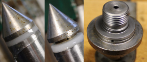 To eliminate all compressible air that would create inaccurate pore pressure measurements, the engineer must fully saturate the pore pressure transducer and filter. He/she fills the cavity between the tip and transducer with silicon oil, waits for all air bubbles to rise to the top, and screws on the tip that has a hole from its bottom to filter side (two connecting holes at 90 degrees) forcing the oil and any air to exit through the hole at the inside of the filter (Figures 2a-c).
Figures 2a-c: Saturating pore pressure transducer
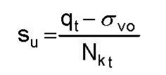
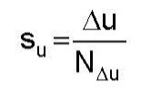
When only oil exits, the engineer confirms a fully saturated pore pressure transducer system. The engineer should use polyethylene porous filters pre-saturated with silicon oil (preferably by the manufacturer). The rigidity of polyethylene prevents the filter from compressing which would cause pore pressure measurement error. Because pore pressures can occur behind the cone tip, the measured tip resistance, qc, is corrected to, qt, using the following formula:
qt = qc + u(1-a), where
qt = the corrected total tip resistance,
qc = the measured tip resistance,
u = pore pressure generated immediately behind the tip,
a = net area ratio
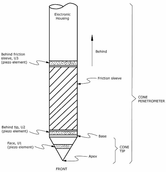
As shown on Figure 3, researchers have measured pore water pressures at 3 locations on the cone penetrometer: 1) on the face of the tip (U1 position), 2) behind the tip (U2 position), and 3) behind the friction sleeve (U3 position). U1 position filters always measure positive pressures but abrade from high stresses in granular soil. U2 position filters generally measure positive pressures and can measure negative pressures in highly over-consolidated soil. With U2 position pore pressure measurements, the engineer corrects the tip stresses for the pore pressure behind the tip as shown on the above equation and as a result prefers this location. Only researchers have used U3 position pore pressure measurements, and it has some difficulties becoming fully saturated. To minimize this pore pressure correction for the U2 position filter, cones should have high net area ratios (ours is 0.8) and this correction is generally less than 2%. Pore pressure can also affect friction measurements. Friction sleeve should have equal end areas at the front and back to eliminate those potential pore pressure corrections, which most cones now have.
Figure 3: Pore pressure filter locations

Figure 4 shows the start of a CPTU sounding with a 10 cm2 piezocone, friction reducer, rubber rod wiper to keep soil below and out of the truck work space, and lateral supporting guide tube to prevent rod buckling.
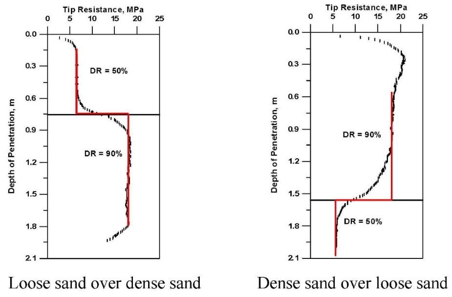
Smaller diameter cones create smaller stress bulbs than larger cones. As a result, smaller cones more accurately measure soil properties at boundaries of differing soil stiffnesses or strengths. 10 cm2 cones more accurately measure soil properties than 15 cm2 cone penetrometers. Ahmadi, Byrne and Campanella (1999) illustrate the importance of smaller projected area CPT probes on the below graphs–smaller stress bulbs more closely follow the correct red lines (Figure 5).
Figure 5: Shows the parasitic effect of larger stress bulbs from cones larger than 10 cm2
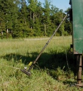
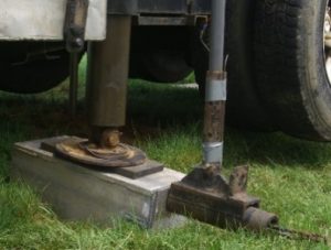 The ASTM downhole seismic method requires an energy source to firmly contact the soil surface from a horizontally offset location and geophones mounted in the probe that can measure the generated shear waves. The energy source consists of a seismic plate and a hammer. Placing the seismic plate just below a leveling jack ensures good coupling between the plate and soil. Placing a rubber pad between the seismic plate and jack makes sure the energy travels into the soil rather than shake the push rig (Areias, Haegeman, Van Impe, 2004). When a sledge hammer, pendulum hammer or automatic hammer strikes the plate horizontally, the plate generates a shear wave with horizontal particle motion and vertical direction of propagation (Figure 6).
Figure 6: Horizontal strike to create seismic shear wave
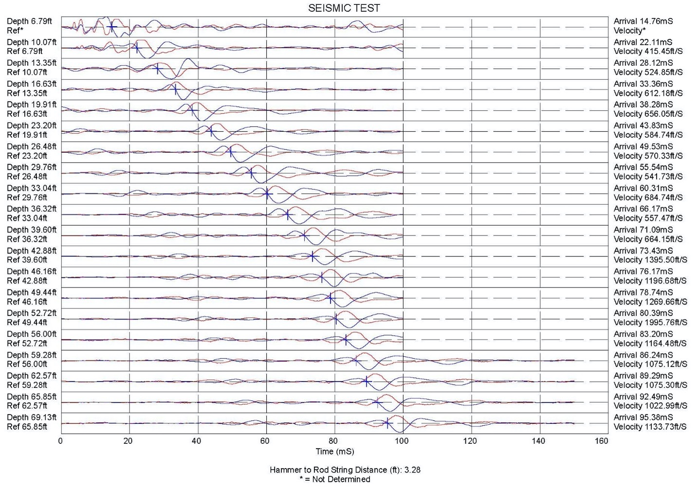
A very accurate and repeatable trigger starts the elapsed time clock the instant that the hammer strikes the plate. The data acquisition computer that simulates an oscilloscope collects and stores the seismic shear wave after each strike. Most CPT systems have only one set of geophones in the probe. After measuring a seismic wave, the engineer must advance the seismic CPT probe and make another horizontal strike. Termed the psuedo-interval method defines this procedure that uses one set of geophones and two depths and sets of strikes/generated waves. He/she generally performs tests at one meter intervals because these intervals conveniently coincide with the end of a push stroke and pausing pushing to add another rod.
The engineer should use either the cross-over method or cross-correlation method to choose the arrival time for each horizontal shear wave (Sully and Campanella, 1995). With the cross-over method, the engineer chooses the time where the wave crosses zero amplitude after the first wave peak or valley. He/she chooses the same location for subsequent waves. The computer calculates the shear wave velocities (Vs) by dividing differences in the hypotenuse travel distances by the differences in arrival times for consecutive test depths. The engineer should check the calculated shear wave velocities to confirm that they make sense with the soil profile and tip resistances. Figure 7 shows an example of sets of seismic waves, where the engineer used the crossover method to find the arrival times. With the cross-correlation method, a computer mathematically shifts the wave at the lower test depth by a delta time until it superimposes on the shear wave at the higher depth. The cross-correlation method works best for measuring systems that have two sets of geophones vertically spaced apart at a constant distance in the probe or module above the probe and one strike creates both sets of waves, also known as the true interval measurement. The engineer can compute the low strain or maximum shear modulus using the following equation:
GMAX = ρ * Vs2
Where GMAX = low strain or maximum shear modulus
ρ = mass density of the soil
Vs = shear wave velocity
Ch = R2 T50/t50
kh = Ch γw/Mh where
Ch = time rate of consolidation in the horizontal direction
R = the radius of the CPT tip
R2 = 0.000318 m2 for a 10 cm2 cone
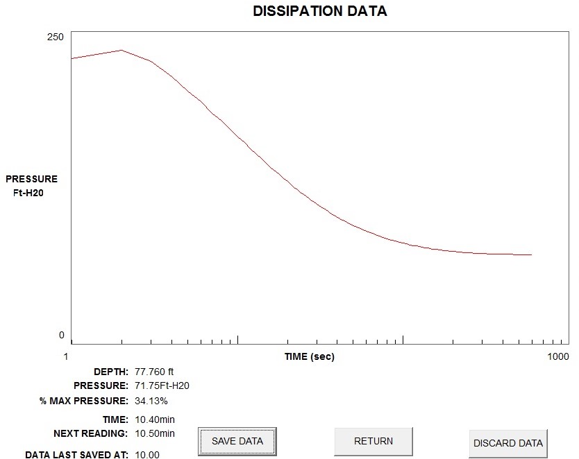
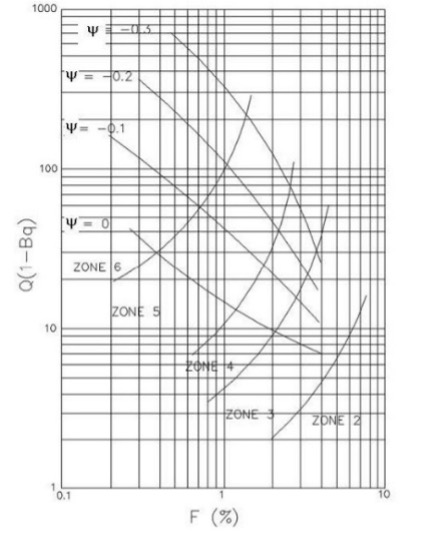
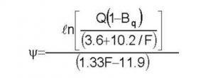
T50=time factor for 50% dissipation from the below family of curves(Battaglio,et.al.,1981)[Figure9]
t50 = time for 50% of dissipation to occur
kh = horizontal coefficient of permeability
γw = unit weight of water
Mh = constrained deformation modulus in the horizontal direction
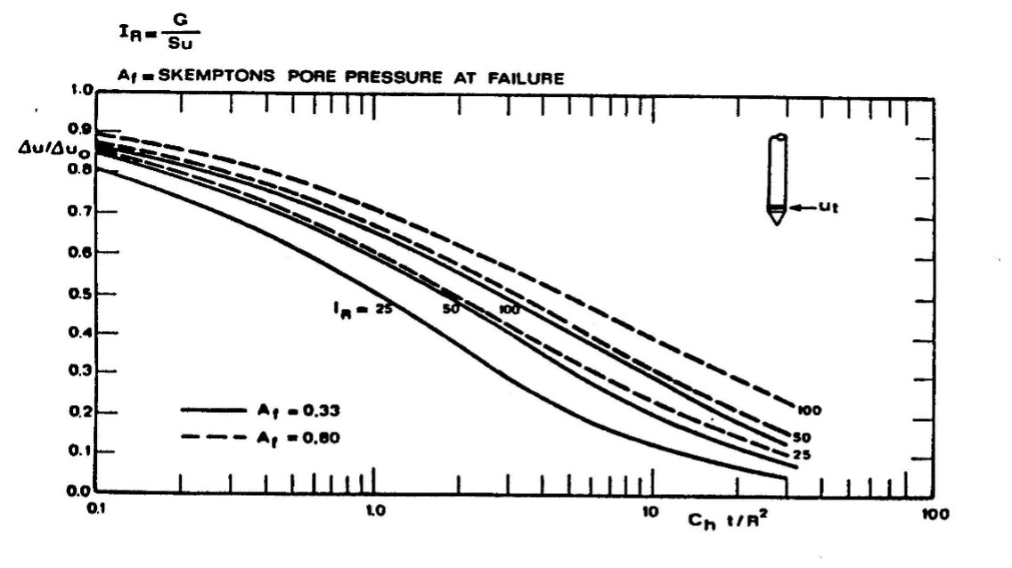
Figure 9: Family of dissipation test curves
Af approximates 0.8 for soft clay, while Af approximates 0.33 for stiff clay. Krage, et. al., 2014 suggests computing the rigidity index, IR using the below formula.
Where IR = rigidity index
GMAX = low strain shear modulus
σ’vo = effective vertical stress
σvo = total vertical stress
qT = corrected tip resistance
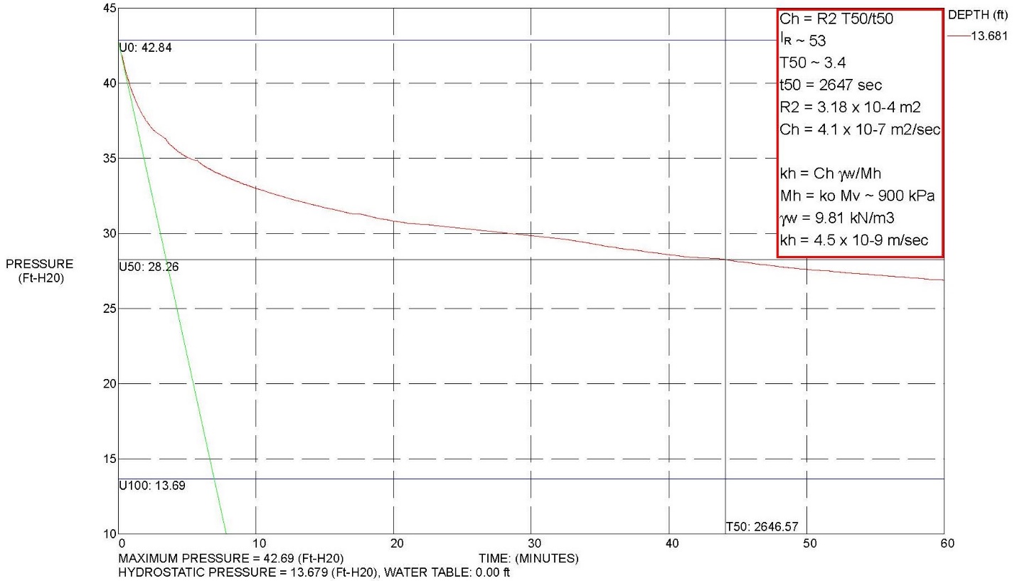
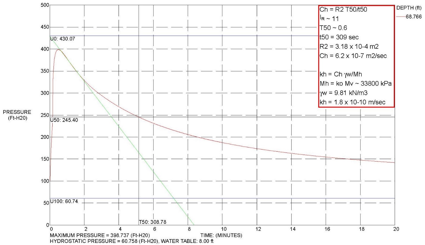 In highly over-consolidated clays, the pore pressure initially increase before decreasing due to the redistribution of excess pore pressures around the tip before they reach an equilibrium state and radial drainage occurs. Figure 10a shows an example of a pore water pressure dissipation test for a normally consolidated clay and figure 10b presents an example of a dissipation for a highly over-consolidated clay.
Figure 10a: Example of processed dissipation test data for normally consolidated clay
Figure 10b: Example of processed dissipation test data for an over-consolidated clay
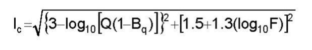

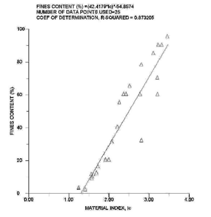
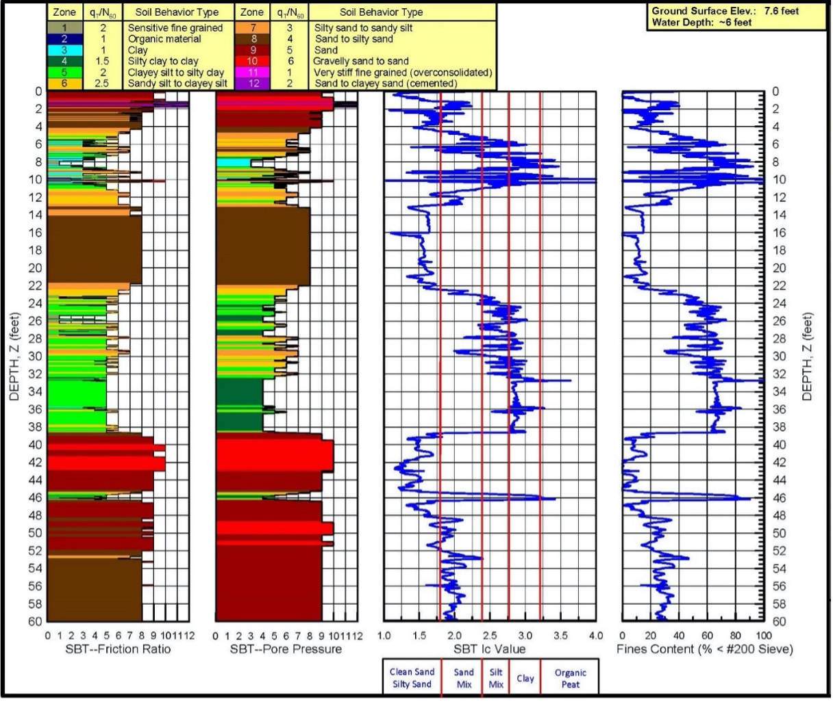
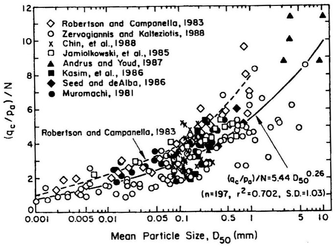
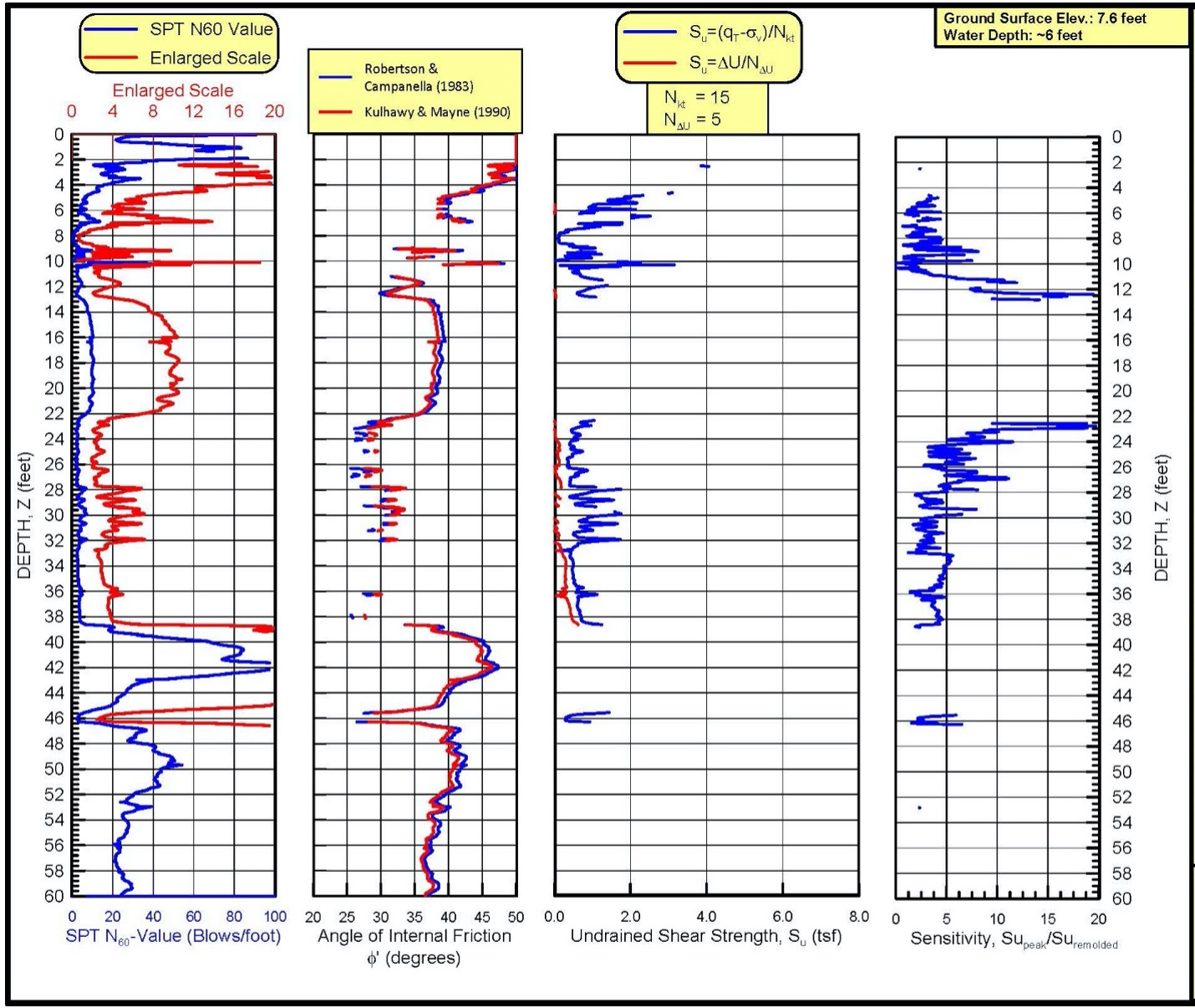
CPT-soil shear strength interpretation: Jefferies and Davies (1993) developed the following equation to compute SPT N60 values based on the Ic value and tip resistance (Figure 16):
Figure 16: SPT/CPT correlation
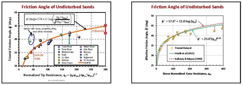
Where the soil behavior type value exceeds 5, the engineer may consider the soil to behave as a cohesionless soil and compute the angle of internal friction using either Robertson and Campanella (1983), Kulhawy and Mayne (1990), and Urielli et. al. (2013) methods (Figure 17a-c). For these methods, φ’ cannot exceed 50 degrees.
For Robertson and Campanella:
φ’ = tan-1((LOG10(qt/σv’)+0.29)/2.68)*180/π
For Kulhawy and Mayne:
φ’ = 17.6+11*LOG10[(qt/σatm)/sq. rt. (σv’/σatm)]
For Uzielli:
φ’ = 25.0o * [(qt/σatm)/sq. rt. (σv’/σatm)]0.10
Robertson and Campanella (1983)
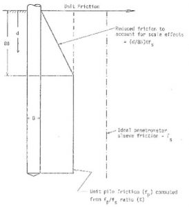
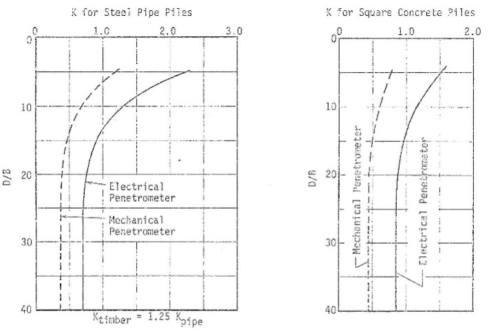
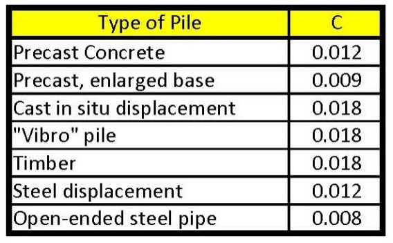
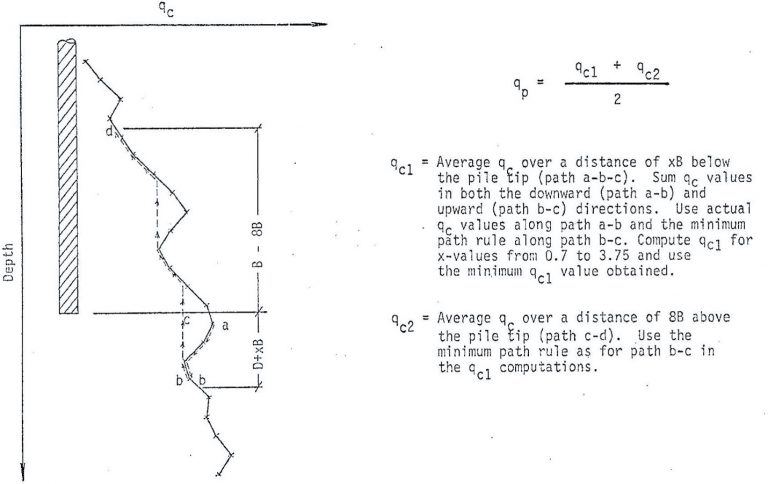
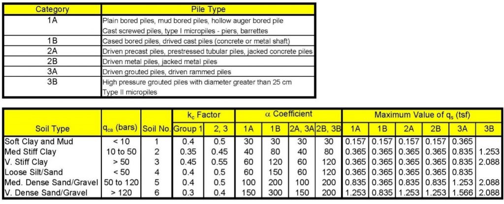
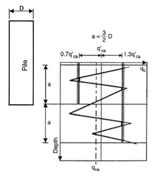 For the LCPC method, the engineer clips the tip resistances that either exceed 1.3 times or less than 0.7 times the average tip resistance in the zone shown in Figure 29. He/she must use an convergence (via a do loop) process because the average value changes after each clipping iteration. The correlation factors depend on the soil type and deep foundation construction method as shown in Figure 30. An Excel spreadsheet that computes vertical pile capacity using the LCPC has the following link LCPC—the macro “qcaverage” clips the extreme values.